
Methodology, Parameters, and Calculations
Parameter definitions, formulas, uncertainty ranges, and data sources.
Keywords
health economics methodology, clinical trial cost analysis, medical research ROI, cost-benefit analysis healthcare, sensitivity analysis, Monte Carlo simulation, DALY calculation, pragmatic clinical trials
Overview
This appendix documents all 152 parameters used in the analysis, organized by type:
- External sources (peer-reviewed): 56
- Calculated values: 70
- Core definitions: 26
Calculated Values
Parameters derived from mathematical formulas and economic models.
Annual Chronic Disease Patients Treated: 982 million people
Note📊 Details
Estimated unique patients receiving chronic disease treatment annually. Derived from IQVIA days of therapy (1.28T) divided by 365 days divided by 2.5 average medications per patient times 70% post-1962 drugs.
Inputs:
- Annual Days of Chronic Disease Therapy 📊: 1.28 trillion days (95% CI: 1 trillion days - 1.5 trillion days)
\[ \begin{gathered} N_{treated} \\ = DOT_{chronic} \times 0.000767 \\ = 1.28T \times 0.000767 \\ = 982M \end{gathered} \]
Methodology:35
? Low confidence
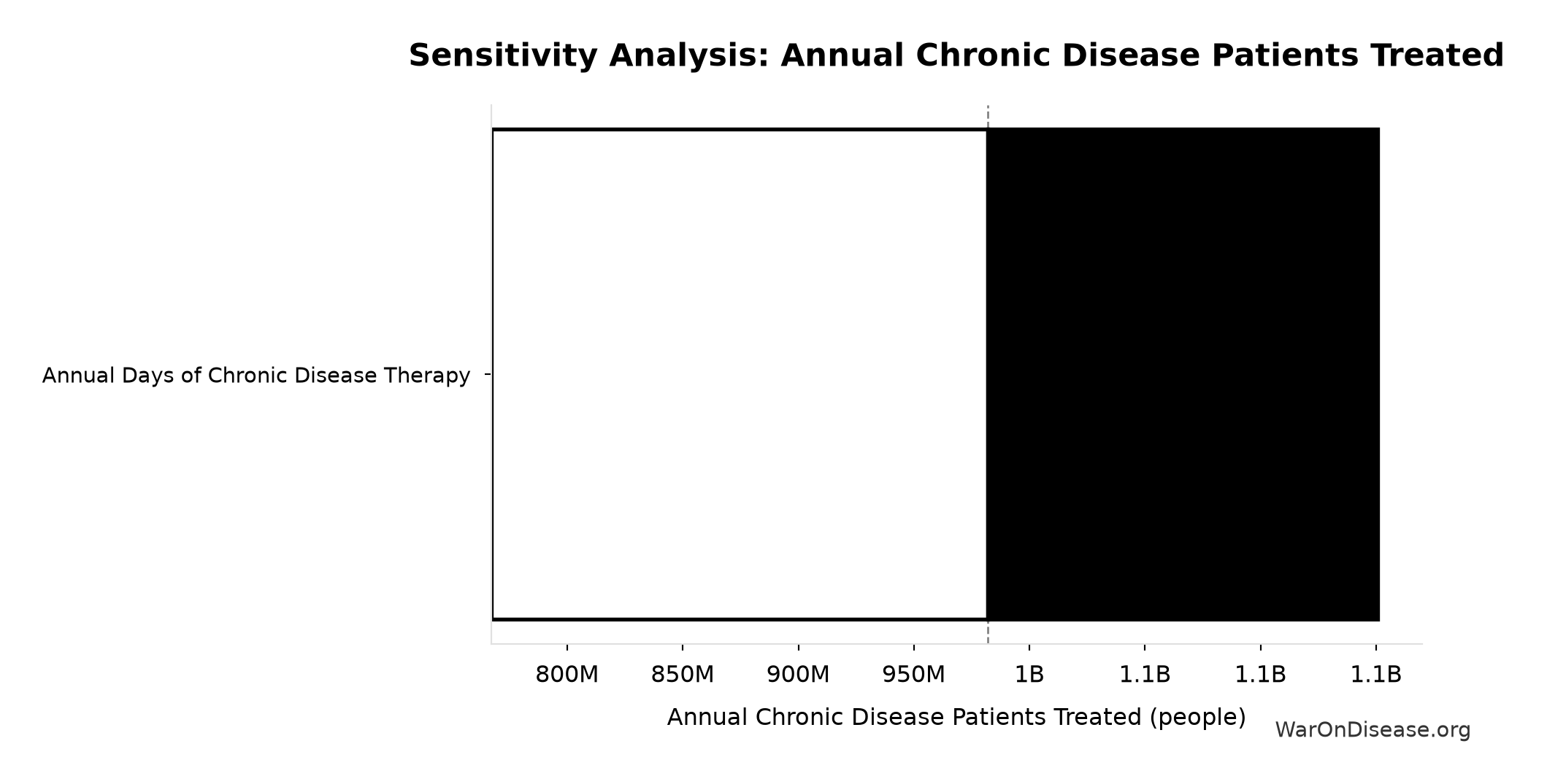
Sensitivity Analysis
Sensitivity Indices for Annual Chronic Disease Patients Treated
Regression-based sensitivity showing which inputs explain the most variance in the output.
| Input Parameter | Sensitivity Coefficient | Interpretation |
|---|---|---|
| Annual Days of Chronic Disease Therapy (days) | 1.0000 | Strong driver |
Interpretation: Standardized coefficients show the change in output (in SD units) per 1 SD change in input. Values near ±1 indicate strong influence; values exceeding ±1 may occur with correlated inputs.
Monte Carlo Distribution
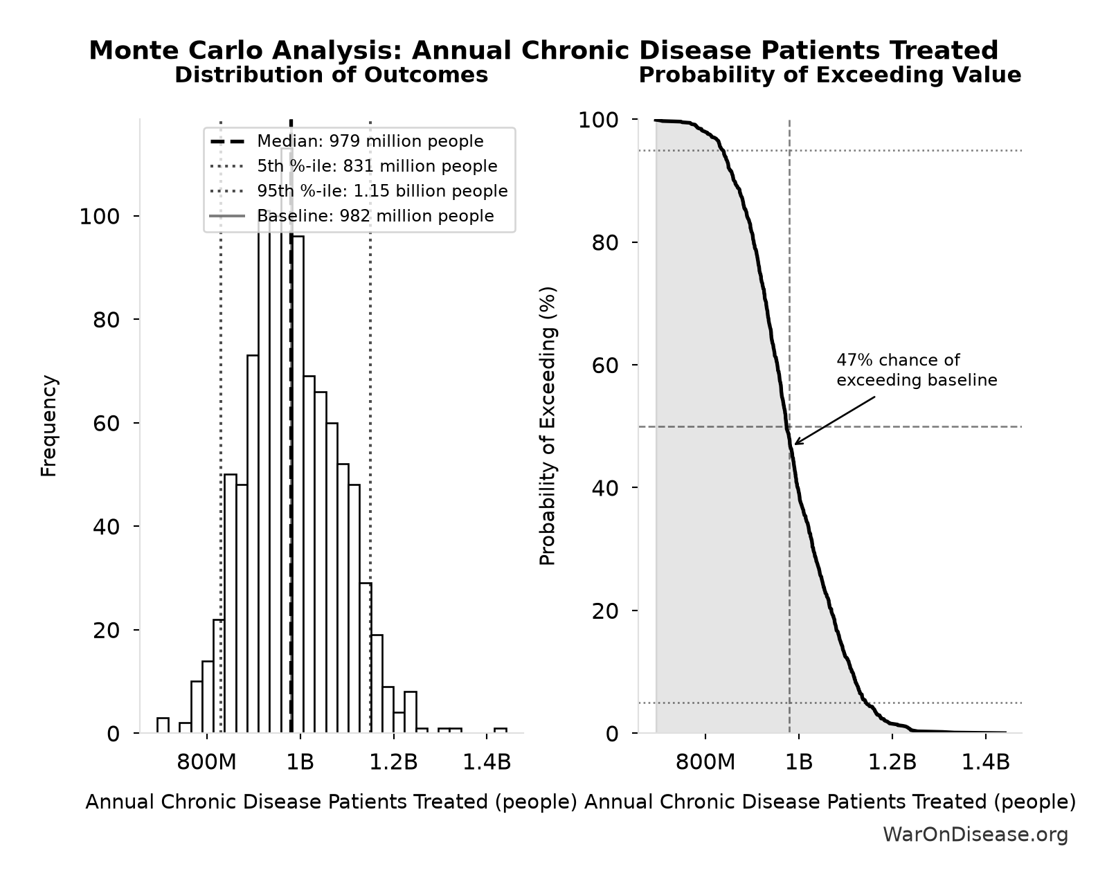
Simulation Results Summary: Annual Chronic Disease Patients Treated
| Statistic | Value |
|---|---|
| Baseline (deterministic) | 982 million |
| Mean (expected value) | 983 million |
| Median (50th percentile) | 979 million |
| Standard Deviation | 98 million |
| 90% Range (5th-95th percentile) | [831 million, 1.15 billion] |
The histogram shows 1,000 of the 10,000 Monte Carlo draws for Annual Chronic Disease Patients Treated; the summary statistics use all 10,000. The exceedance curve (right) shows the probability of the outcome exceeding any given value.
Exceedance Probability
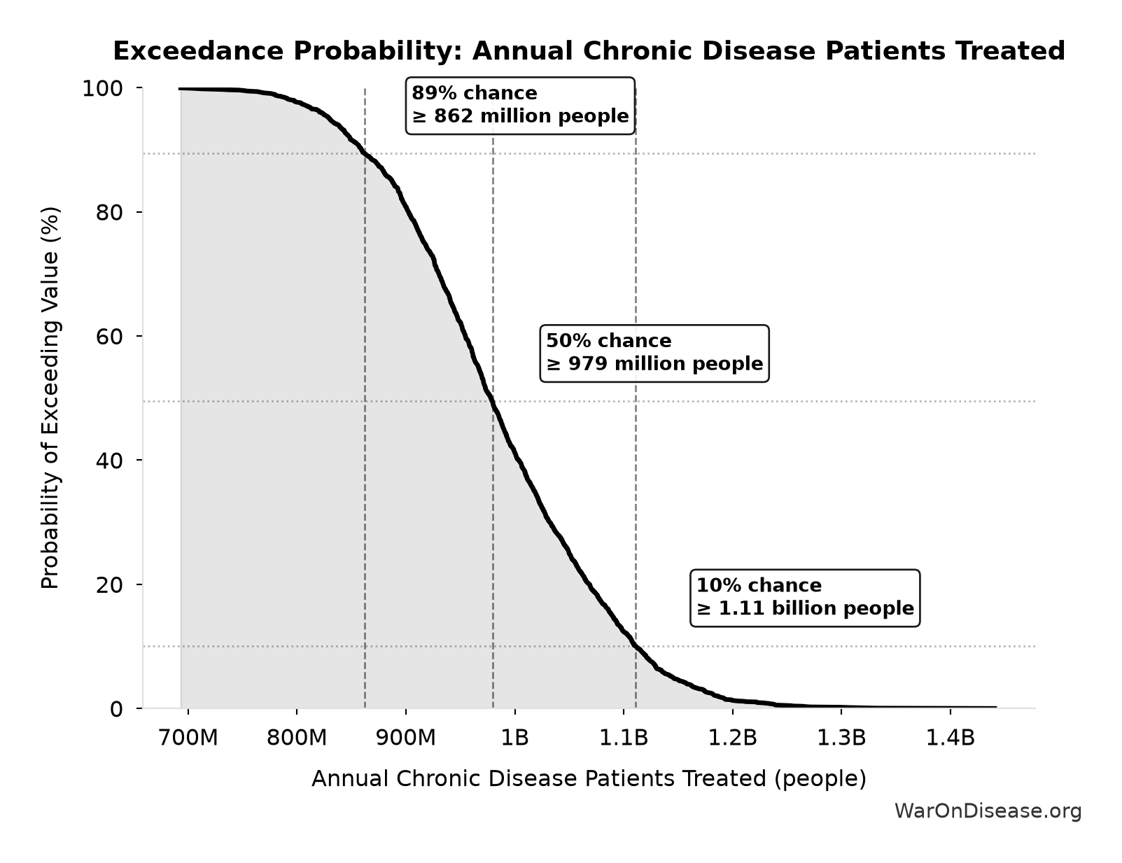
This exceedance probability chart shows the likelihood that Annual Chronic Disease Patients Treated will exceed any given threshold. The higher the curve at a threshold, the more likely the value exceeds it.
Combination Therapy Space: 45.1 billion combinations
Note📊 Details
Total combination therapy space (pairwise drug combinations × diseases). Standard in oncology, HIV, cardiology.
Inputs:
- Pairwise Drug Combinations 🔢: 45.1 million combinations
- Trial-Relevant Diseases: 1,000 diseases (95% CI: 800 diseases - 1,200 diseases)
\[ \begin{gathered} Space_{combo} \\ = N_{combo} \times N_{diseases,trial} \\ = 45.1M \times 1{,}000 \\ = 45.1B \end{gathered} \] where: \[ N_{combo} = \frac{N_{safe} \cdot (N_{safe} - 1)}{2} \] ✓ High confidence
Sensitivity Analysis
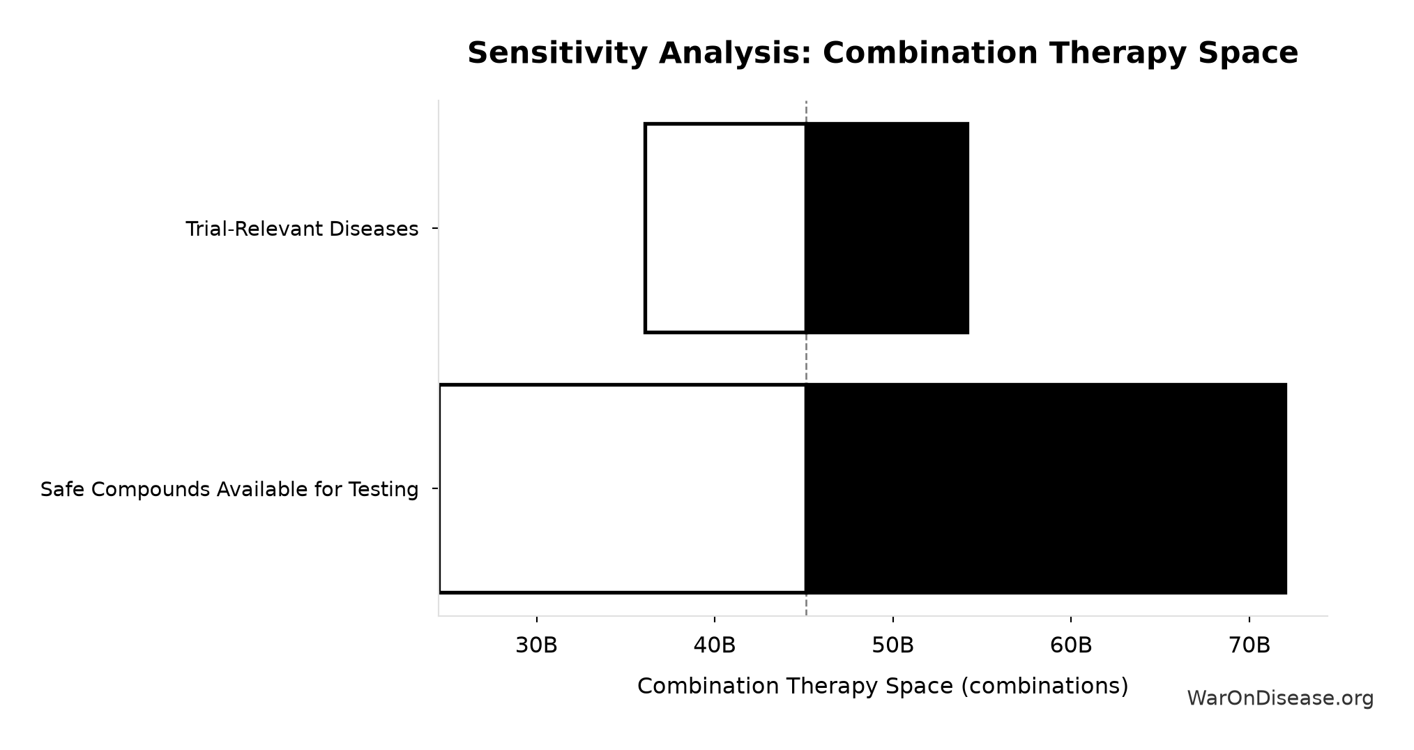
Sensitivity Indices for Combination Therapy Space
Regression-based sensitivity showing which inputs explain the most variance in the output.
| Input Parameter | Sensitivity Coefficient | Interpretation |
|---|---|---|
| Pairwise Drug Combinations (combinations) | 0.9212 | Strong driver |
| Trial-Relevant Diseases (diseases) | 0.3584 | Moderate driver |
Interpretation: Standardized coefficients show the change in output (in SD units) per 1 SD change in input. Values near ±1 indicate strong influence; values exceeding ±1 may occur with correlated inputs.
Monte Carlo Distribution
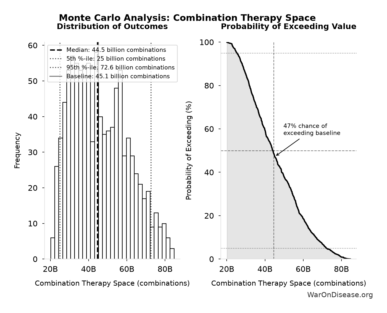
Simulation Results Summary: Combination Therapy Space
| Statistic | Value |
|---|---|
| Baseline (deterministic) | 45.1 billion |
| Mean (expected value) | 46.1 billion |
| Median (50th percentile) | 44.5 billion |
| Standard Deviation | 14.9 billion |
| 90% Range (5th-95th percentile) | [25 billion, 72.6 billion] |
The histogram shows 1,000 of the 10,000 Monte Carlo draws for Combination Therapy Space; the summary statistics use all 10,000. The exceedance curve (right) shows the probability of the outcome exceeding any given value.
Exceedance Probability
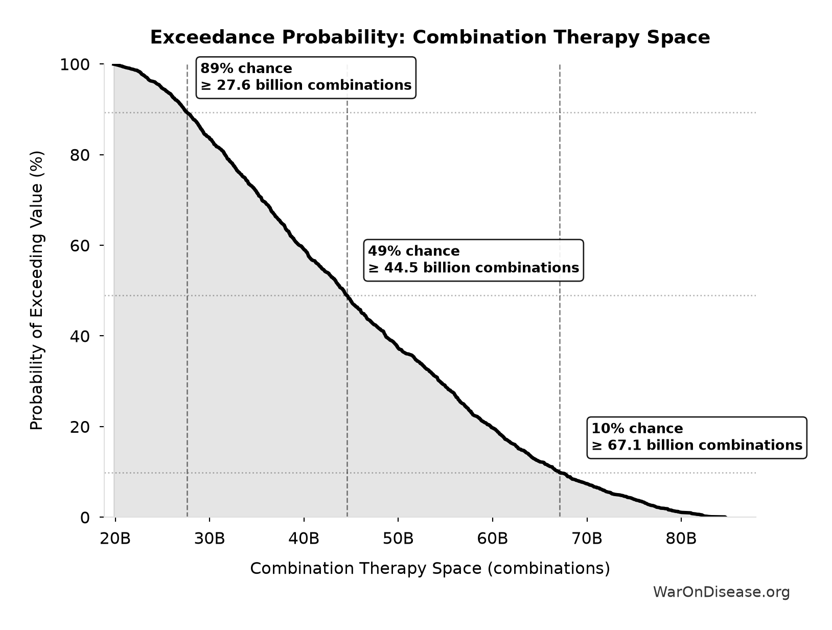
This exceedance probability chart shows the likelihood that Combination Therapy Space will exceed any given threshold. The higher the curve at a threshold, the more likely the value exceeds it.
Pairwise Drug Combinations: 45.1 million combinations
Note📊 Details
Unique pairwise drug combinations from known safe compounds (n choose 2)
Inputs:
- Safe Compounds Available for Testing: 9,500 compounds (95% CI: 7,000 compounds - 12,000 compounds)
\[ N_{combo} = \frac{N_{safe} \cdot (N_{safe} - 1)}{2} \]
✓ High confidence
Sensitivity Analysis
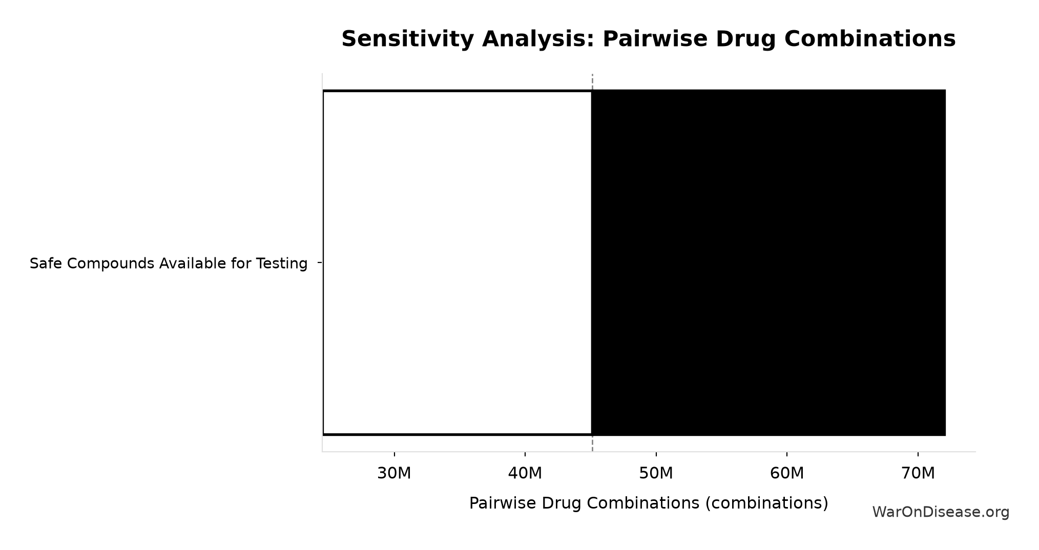
Sensitivity Indices for Pairwise Drug Combinations
Regression-based sensitivity showing which inputs explain the most variance in the output.
| Input Parameter | Sensitivity Coefficient | Interpretation |
|---|---|---|
| Safe Compounds Available for Testing (compounds) | 0.9977 | Strong driver |
Interpretation: Standardized coefficients show the change in output (in SD units) per 1 SD change in input. Values near ±1 indicate strong influence; values exceeding ±1 may occur with correlated inputs.
Monte Carlo Distribution
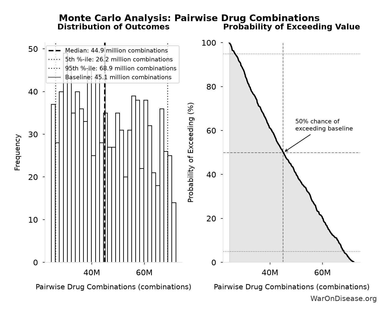
Simulation Results Summary: Pairwise Drug Combinations
| Statistic | Value |
|---|---|
| Baseline (deterministic) | 45.1 million |
| Mean (expected value) | 46.1 million |
| Median (50th percentile) | 44.9 million |
| Standard Deviation | 13.7 million |
| 90% Range (5th-95th percentile) | [26.2 million, 68.9 million] |
The histogram shows 1,000 of the 10,000 Monte Carlo draws for Pairwise Drug Combinations; the summary statistics use all 10,000. The exceedance curve (right) shows the probability of the outcome exceeding any given value.
Exceedance Probability
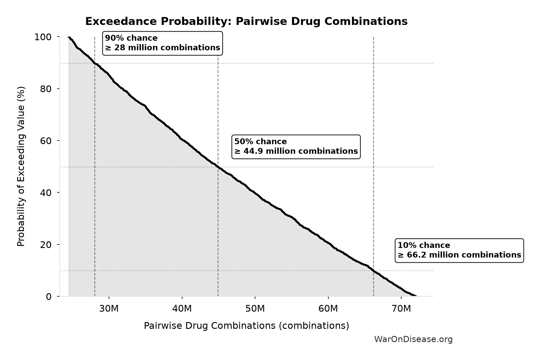
This exceedance probability chart shows the likelihood that Pairwise Drug Combinations will exceed any given threshold. The higher the curve at a threshold, the more likely the value exceeds it.
Combination Therapy Exploration Time (Current): 13.7 million years
Note📊 Details
Years to test all pairwise drug combinations at current trial capacity. Combination therapy is standard in oncology, HIV, cardiology.
Inputs:
- Combination Therapy Space 🔢: 45.1 billion combinations
- Current Global Clinical Trials per Year 📊: 3,300 trials/year (95% CI: 2,640 trials/year - 3,960 trials/year)
\[ \begin{gathered} T_{explore,combo} \\ = \frac{Space_{combo}}{Trials_{ann,curr}} \\ = \frac{45.1B}{3{,}300} \\ = 13.7M \end{gathered} \] where: \[ \begin{gathered} Space_{combo} \\ = N_{combo} \times N_{diseases,trial} \\ = 45.1M \times 1{,}000 \\ = 45.1B \end{gathered} \] where: \[ N_{combo} = \frac{N_{safe} \cdot (N_{safe} - 1)}{2} \] ✓ High confidence
Sensitivity Analysis
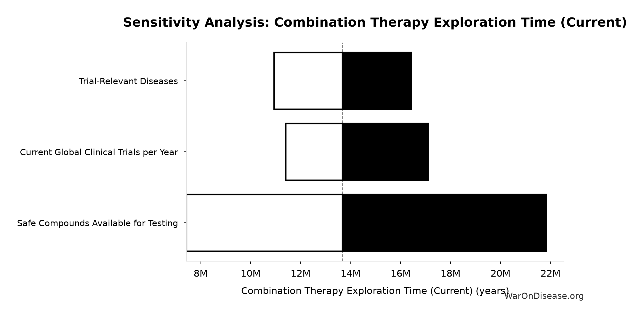
Sensitivity Indices for Combination Therapy Exploration Time (Current)
Regression-based sensitivity showing which inputs explain the most variance in the output.
| Input Parameter | Sensitivity Coefficient | Interpretation |
|---|---|---|
| Combination Therapy Space (combinations) | 0.9556 | Strong driver |
| Current Global Clinical Trials per Year (trials/year) | -0.2867 | Weak driver |
Interpretation: Standardized coefficients show the change in output (in SD units) per 1 SD change in input. Values near ±1 indicate strong influence; values exceeding ±1 may occur with correlated inputs.
Monte Carlo Distribution
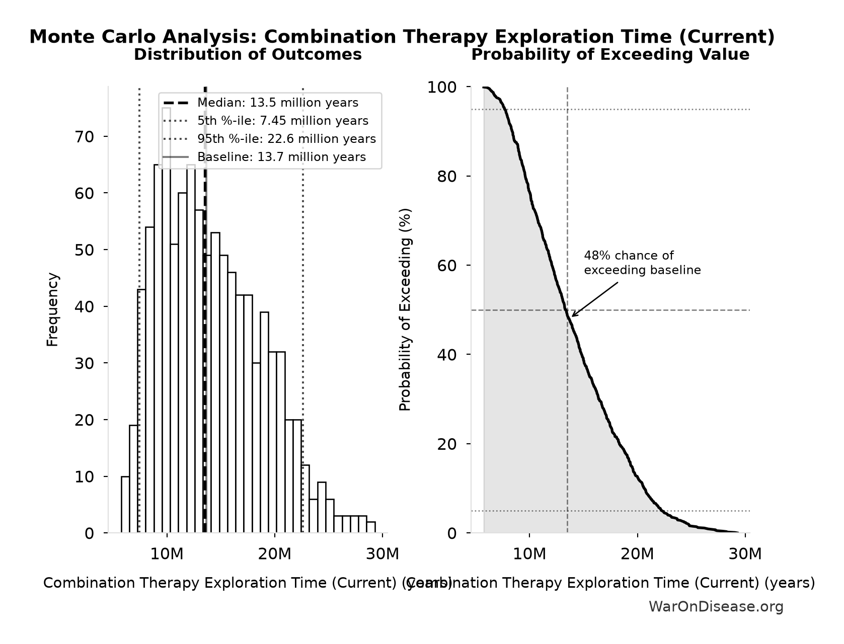
Simulation Results Summary: Combination Therapy Exploration Time (Current)
| Statistic | Value |
|---|---|
| Baseline (deterministic) | 13.7 million |
| Mean (expected value) | 14.1 million |
| Median (50th percentile) | 13.5 million |
| Standard Deviation | 4.76 million |
| 90% Range (5th-95th percentile) | [7.45 million, 22.6 million] |
The histogram shows 1,000 of the 10,000 Monte Carlo draws for Combination Therapy Exploration Time (Current); the summary statistics use all 10,000. The exceedance curve (right) shows the probability of the outcome exceeding any given value.
Exceedance Probability
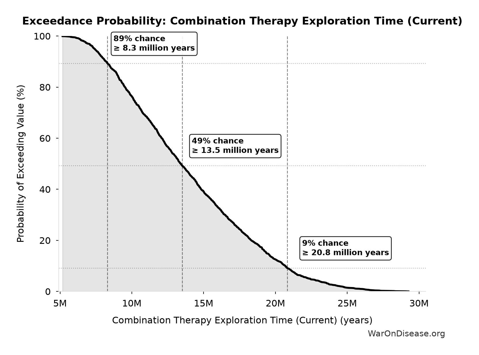
This exceedance probability chart shows the likelihood that Combination Therapy Exploration Time (Current) will exceed any given threshold. The higher the curve at a threshold, the more likely the value exceeds it.
Known Safe Exploration Time (Current): 2,879 years
Note📊 Details
Years to test all known safe drug-disease combinations at current global trial capacity
Inputs:
- Possible Drug-Disease Combinations 🔢: 9.5 million combinations
- Current Global Clinical Trials per Year 📊: 3,300 trials/year (95% CI: 2,640 trials/year - 3,960 trials/year)
\[ \begin{gathered} T_{explore,safe} \\ = \frac{N_{combos}}{Trials_{ann,curr}} \\ = \frac{9.5M}{3{,}300} \\ = 2{,}880 \end{gathered} \] where: \[ \begin{gathered} N_{combos} \\ = N_{safe} \times N_{diseases,trial} \\ = 9{,}500 \times 1{,}000 \\ = 9.5M \end{gathered} \] ✓ High confidence
Sensitivity Analysis
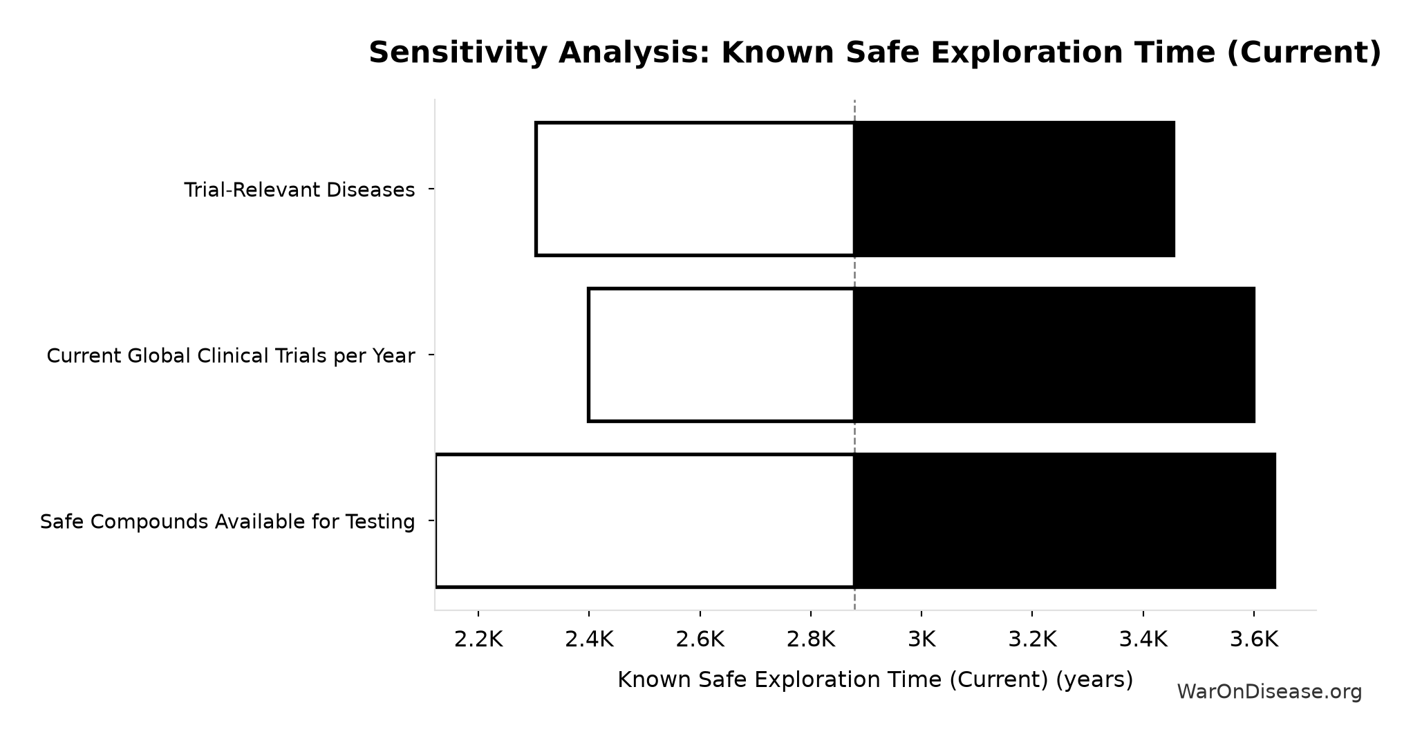
Sensitivity Indices for Known Safe Exploration Time (Current)
Regression-based sensitivity showing which inputs explain the most variance in the output.
| Input Parameter | Sensitivity Coefficient | Interpretation |
|---|---|---|
| Possible Drug-Disease Combinations (combinations) | 0.8940 | Strong driver |
| Current Global Clinical Trials per Year (trials/year) | -0.4473 | Moderate driver |
Interpretation: Standardized coefficients show the change in output (in SD units) per 1 SD change in input. Values near ±1 indicate strong influence; values exceeding ±1 may occur with correlated inputs.
Monte Carlo Distribution
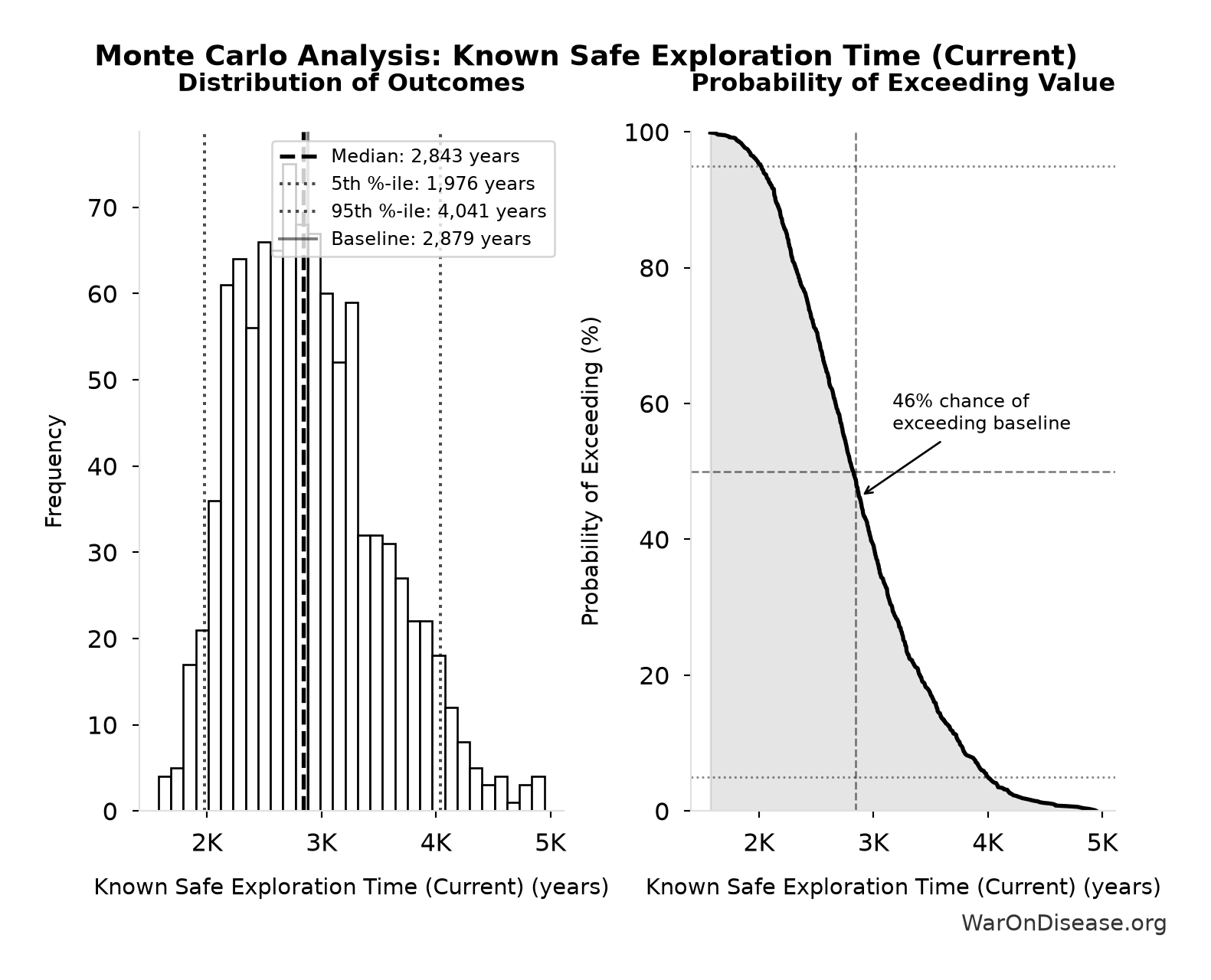
Simulation Results Summary: Known Safe Exploration Time (Current)
| Statistic | Value |
|---|---|
| Baseline (deterministic) | 2,879 |
| Mean (expected value) | 2,904 |
| Median (50th percentile) | 2,843 |
| Standard Deviation | 628 |
| 90% Range (5th-95th percentile) | [1,976, 4,041] |
The histogram shows 1,000 of the 10,000 Monte Carlo draws for Known Safe Exploration Time (Current); the summary statistics use all 10,000. The exceedance curve (right) shows the probability of the outcome exceeding any given value.
Exceedance Probability
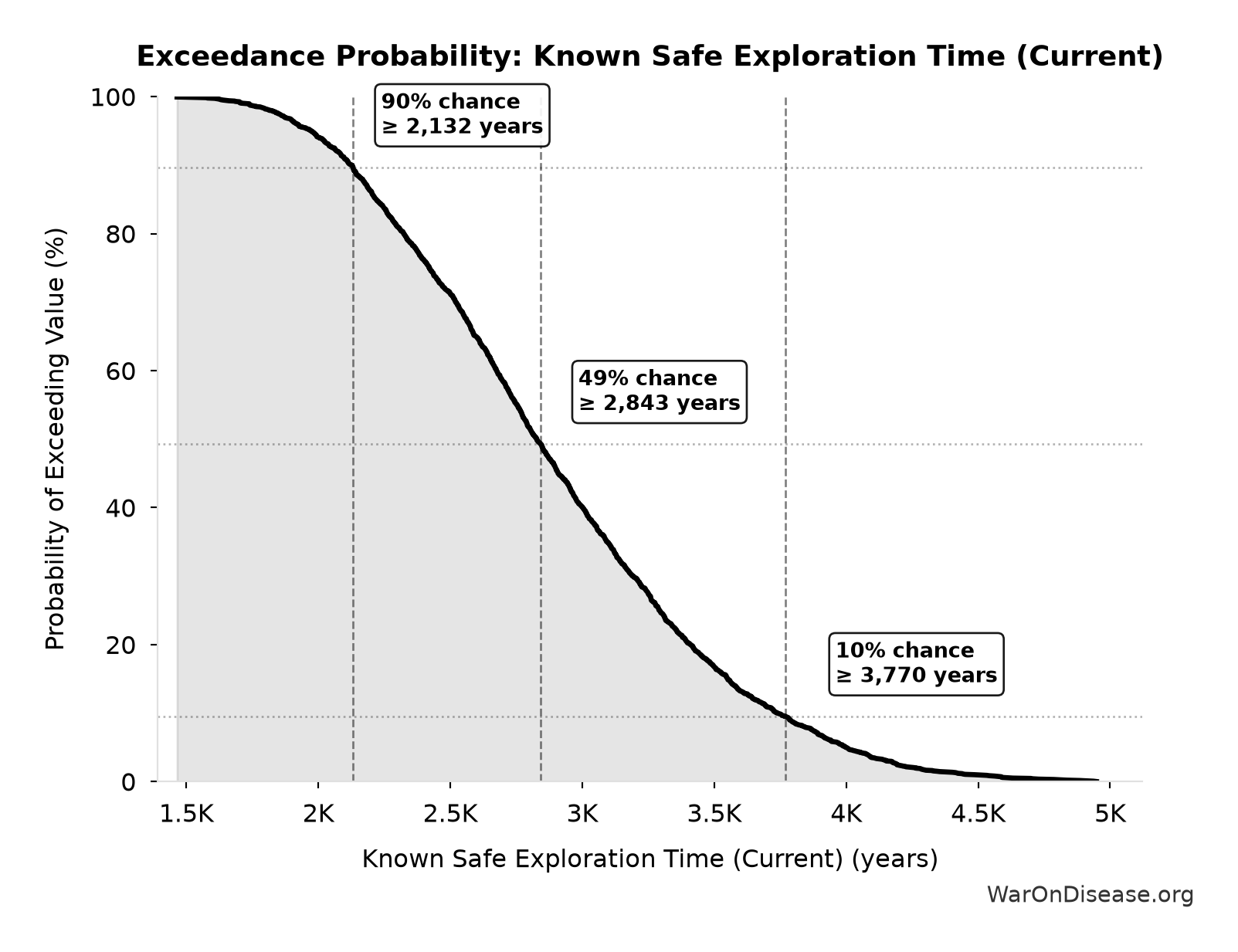
This exceedance probability chart shows the likelihood that Known Safe Exploration Time (Current) will exceed any given threshold. The higher the curve at a threshold, the more likely the value exceeds it.
Total Annual Pragmatic Trial Platform Operational Costs: $40 million
Note📊 Details
Total annual pragmatic trial platform operational costs (sum of all components: platform + staff + infra + regulatory + community)
Inputs:
- Pragmatic Trial Platform Maintenance Costs: $15 million (95% CI: $10 million - $22 million)
- Pragmatic Trial Platform Staff Costs: $10 million (95% CI: $7 million - $15 million)
- Pragmatic Trial Platform Infrastructure Costs: $8 million (95% CI: $5 million - $12 million)
- Pragmatic Trial Platform Regulatory Coordination Costs: $5 million (95% CI: $3 million - $8 million)
- Pragmatic Trial Platform Community Support Costs: $2 million (95% CI: $1 million - $3 million)
\[ \begin{gathered} OPEX_{trial} \\ = Cost_{platform} + Cost_{staff} + Cost_{infra} \\ + Cost_{regulatory} + Cost_{community} \\ = \$15M + \$10M + \$8M + \$5M + \$2M \\ = \$40M \end{gathered} \]
✓ High confidence
Sensitivity Analysis
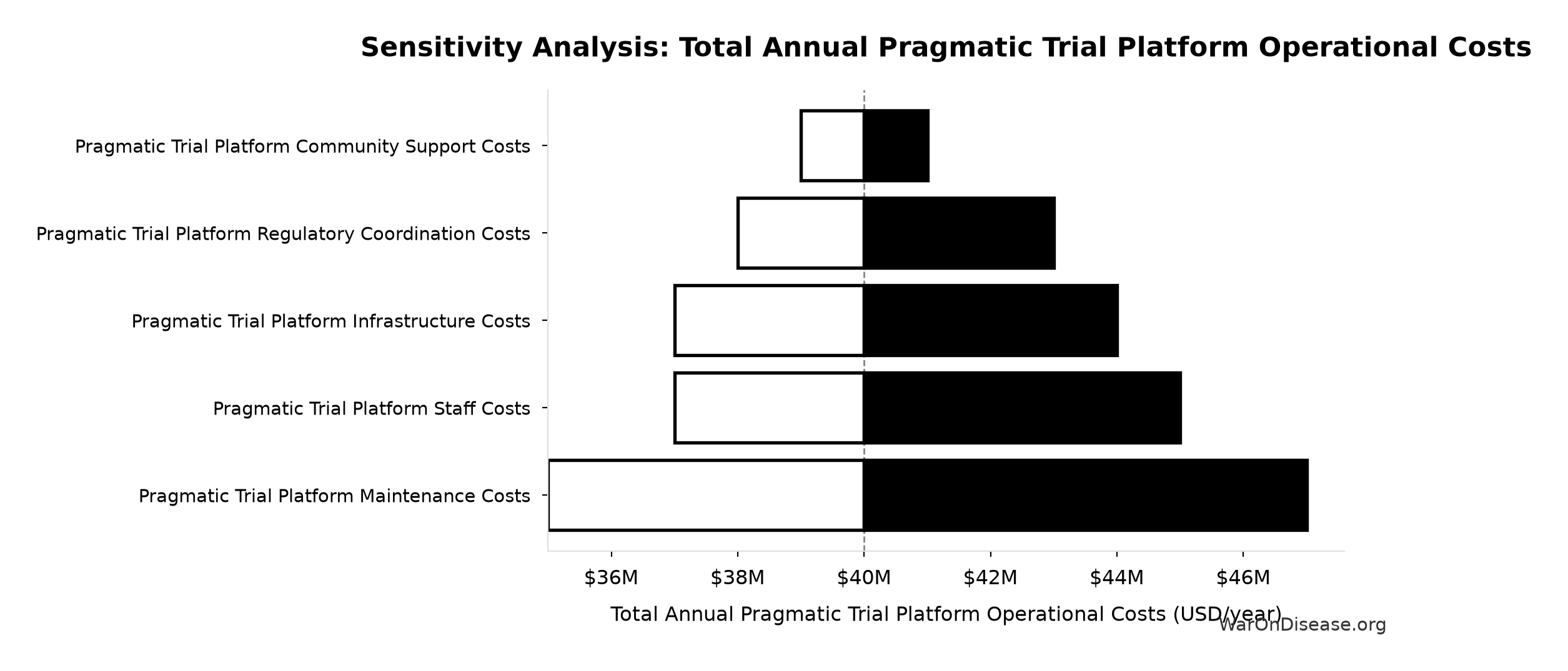
Sensitivity Indices for Total Annual Pragmatic Trial Platform Operational Costs
Regression-based sensitivity showing which inputs explain the most variance in the output.
| Input Parameter | Sensitivity Coefficient | Interpretation |
|---|---|---|
| Pragmatic Trial Platform Maintenance Costs (USD/year) | 0.7128 | Strong driver |
| Pragmatic Trial Platform Staff Costs (USD/year) | 0.4775 | Moderate driver |
| Pragmatic Trial Platform Infrastructure Costs (USD/year) | 0.4127 | Moderate driver |
| Pragmatic Trial Platform Regulatory Coordination Costs (USD/year) | 0.2936 | Weak driver |
| Pragmatic Trial Platform Community Support Costs (USD/year) | 0.1156 | Weak driver |
Interpretation: Standardized coefficients show the change in output (in SD units) per 1 SD change in input. Values near ±1 indicate strong influence; values exceeding ±1 may occur with correlated inputs.
Monte Carlo Distribution
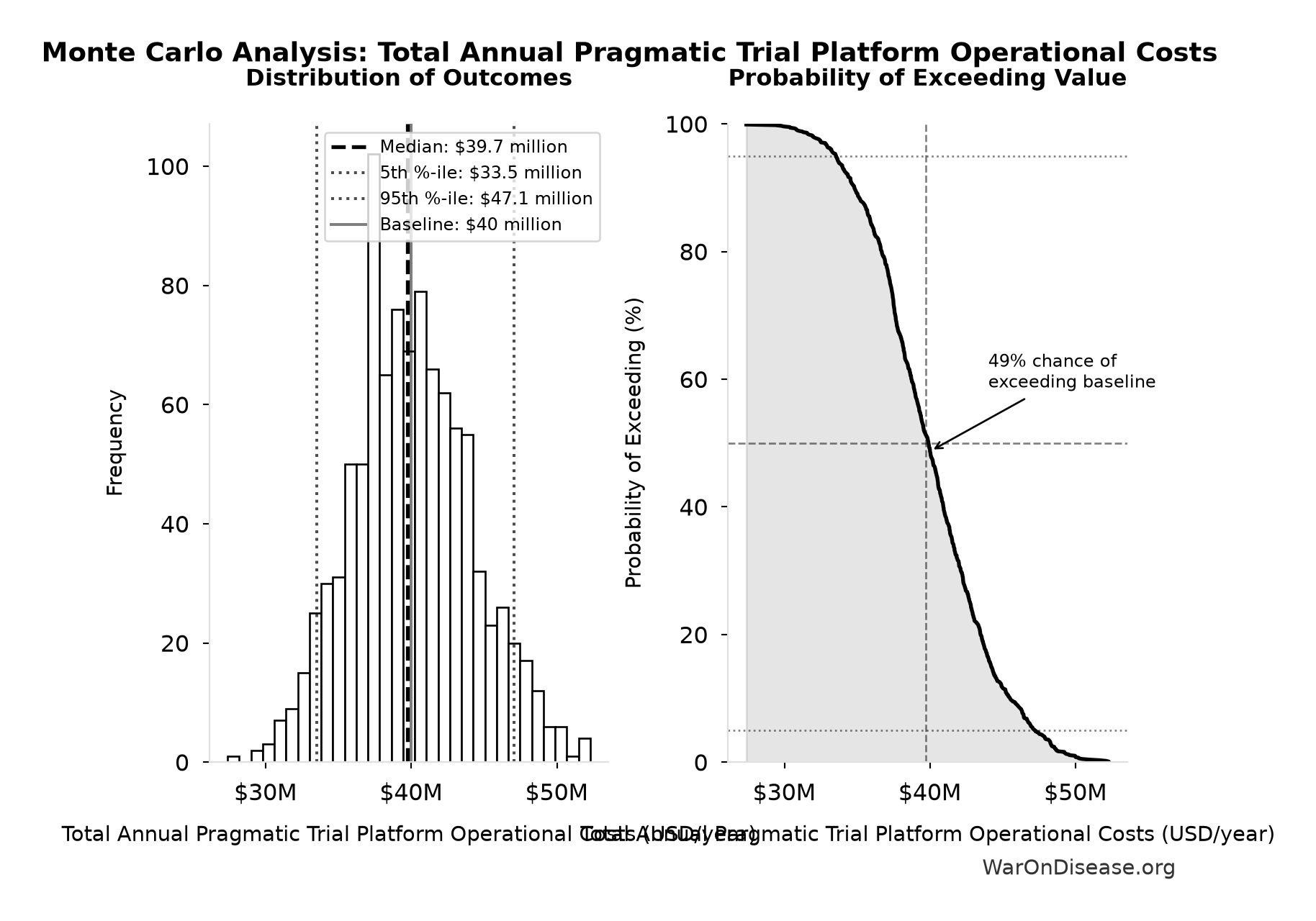
Simulation Results Summary: Total Annual Pragmatic Trial Platform Operational Costs
| Statistic | Value |
|---|---|
| Baseline (deterministic) | $40 million |
| Mean (expected value) | $39.9 million |
| Median (50th percentile) | $39.7 million |
| Standard Deviation | $4.09 million |
| 90% Range (5th-95th percentile) | [$33.5 million, $47.1 million] |
The histogram shows 1,000 of the 10,000 Monte Carlo draws for Total Annual Pragmatic Trial Platform Operational Costs; the summary statistics use all 10,000. The exceedance curve (right) shows the probability of the outcome exceeding any given value.
Exceedance Probability
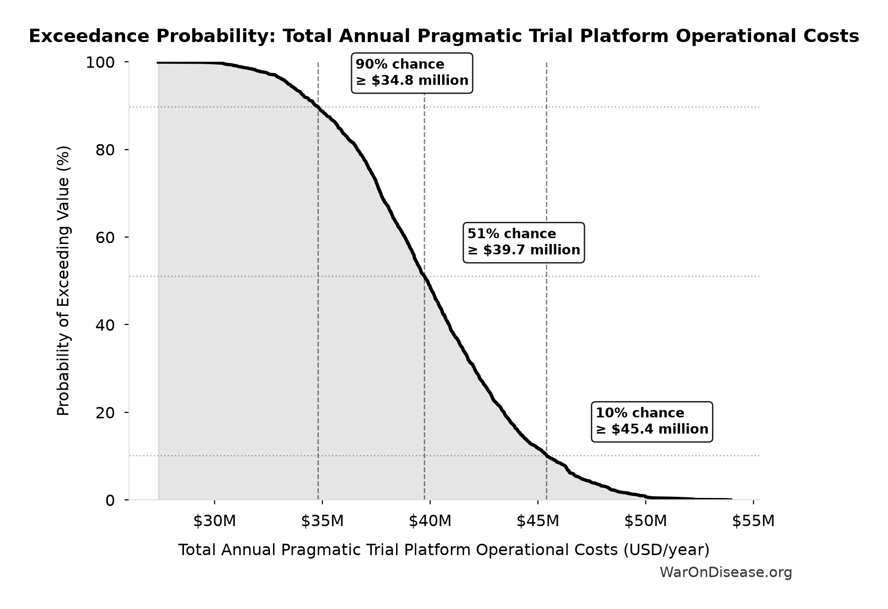
This exceedance probability chart shows the likelihood that Total Annual Pragmatic Trial Platform Operational Costs will exceed any given threshold. The higher the curve at a threshold, the more likely the value exceeds it.
Annual R&D Savings from Pragmatic Trials: $40.5 billion
Note📊 Details
Annual benefit from pragmatic trial R&D savings: trial cost reduction applied to the Phase 2/3 efficacy share of global trial spending (Phase 1 safety trials retain traditional design and cost)
Inputs:
- Annual Global Spending on Clinical Trials 📊: $60 billion (95% CI: $50 billion - $75 billion)
- Phase 2/3 Share of Clinical Trial Costs 📊: 69% (SE: ±5%)
- Pragmatic Trial Cost Reduction Percentage 🔢: 97.7%
\[ \begin{gathered} Benefit_{RD,ann} \\ = Spending_{trials} \times Pct_{P2+P3} \times Reduce_{pct} \\ = \$60B \times 69\% \times 97.7\% \\ = \$40.5B \end{gathered} \] where: \[ \begin{gathered} Reduce_{pct} \\ = 1 - \frac{Cost_{pragmatic,pt}}{Cost_{P3,pt}} \\ = 1 - \frac{\$929}{\$41K} \\ = 97.7\% \end{gathered} \] ✓ High confidence
Sensitivity Analysis
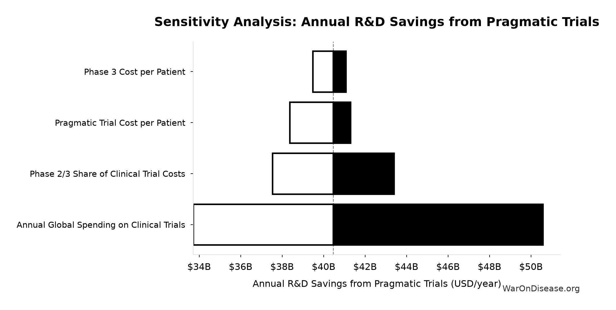
Sensitivity Indices for Annual R&D Savings from Pragmatic Trials
Regression-based sensitivity showing which inputs explain the most variance in the output.
| Input Parameter | Sensitivity Coefficient | Interpretation |
|---|---|---|
| Annual Global Spending on Clinical Trials (USD) | 0.8666 | Strong driver |
| Phase 2/3 Share of Clinical Trial Costs (percentage) | 0.4697 | Moderate driver |
| Pragmatic Trial Cost Reduction Percentage (percentage) | 0.1657 | Weak driver |
Interpretation: Standardized coefficients show the change in output (in SD units) per 1 SD change in input. Values near ±1 indicate strong influence; values exceeding ±1 may occur with correlated inputs.
Monte Carlo Distribution
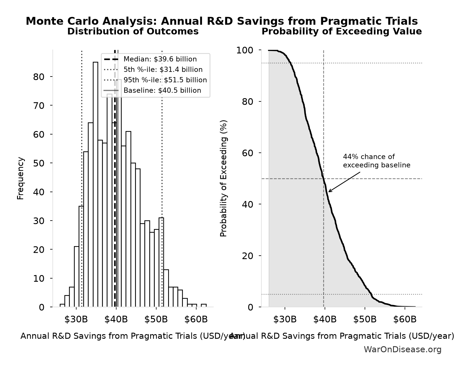
Simulation Results Summary: Annual R&D Savings from Pragmatic Trials
| Statistic | Value |
|---|---|
| Baseline (deterministic) | $40.5 billion |
| Mean (expected value) | $40.3 billion |
| Median (50th percentile) | $39.6 billion |
| Standard Deviation | $6.21 billion |
| 90% Range (5th-95th percentile) | [$31.4 billion, $51.5 billion] |
The histogram shows 1,000 of the 10,000 Monte Carlo draws for Annual R&D Savings from Pragmatic Trials; the summary statistics use all 10,000. The exceedance curve (right) shows the probability of the outcome exceeding any given value.
Exceedance Probability
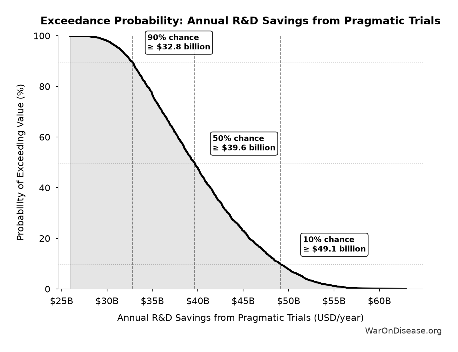
This exceedance probability chart shows the likelihood that Annual R&D Savings from Pragmatic Trials will exceed any given threshold. The higher the curve at a threshold, the more likely the value exceeds it.
Direct Pragmatic Trial Funding Cost per DALY: $0.842
Note📊 Details
Cost per DALY at direct funding level for the therapeutic space exploration period. Still highly cost-effective vs bed nets.
Inputs:
- Direct Pragmatic Trial Funding NPV (Exploration Period) 🔢: $476 billion
- Total DALYs from Elimination of Efficacy Lag Plus Earlier Treatment Discovery from Higher Trial Throughput 🔢: 565 billion DALYs
\[ \begin{gathered} Cost_{direct,DALY} \\ = \frac{NPV_{direct}}{DALYs_{max}} \\ = \frac{\$476B}{565B} \\ = \$0.842 \end{gathered} \] where: \[ \begin{gathered} NPV_{direct} \\ = \frac{T_{queue,trial}}{Funding_{trial,ref} \times r_{discount}} \\ = \frac{36}{\$21.8B \times 3\%} \\ = \$476B \end{gathered} \] where: \[ \begin{gathered} T_{queue,trial} \\ = \frac{T_{queue,SQ}}{k_{capacity}} \\ = \frac{443}{12.3} \\ = 36 \end{gathered} \] where: \[ \begin{gathered} T_{queue,SQ} \\ = \frac{N_{untreated}}{Treatments_{new,ann}} \\ = \frac{6{,}650}{15} \\ = 443 \end{gathered} \] where: \[ \begin{gathered} N_{untreated} \\ = N_{rare} \times 0.95 \\ = 7{,}000 \times 0.95 \\ = 6{,}650 \end{gathered} \] where: \[ \begin{gathered} k_{capacity} \\ = \frac{N_{fundable,ref}}{Slots_{curr}} \\ = \frac{23.4M}{1.9M} \\ = 12.3 \end{gathered} \] where: \[ \begin{gathered} N_{fundable,ref} \\ = \frac{Subsidies_{trial,ref}}{Cost_{pragmatic,pt}} \\ = \frac{\$21.8B}{\$929} \\ = 23.4M \end{gathered} \] where: \[ \begin{gathered} Subsidies_{trial,ref} \\ = Funding_{trial,ref} - OPEX_{trial} \\ = \$21.8B - \$40M \\ = \$21.8B \end{gathered} \] where: \[ \begin{gathered} OPEX_{trial} \\ = Cost_{platform} + Cost_{staff} + Cost_{infra} \\ + Cost_{regulatory} + Cost_{community} \\ = \$15M + \$10M + \$8M + \$5M + \$2M \\ = \$40M \end{gathered} \] where: \[ \begin{gathered} DALYs_{max} \\ = DALYs_{global,ann} \times Pct_{avoid,DALY} \times T_{accel,max} \\ = 2.88B \times 92.6\% \times 212 \\ = 565B \end{gathered} \] where: \[ T_{accel,max} = T_{accel} + T_{lag} = 204 + 8.2 = 212 \] where: \[ \begin{gathered} T_{accel} \\ = T_{first,SQ} \times \left(1 - \frac{1}{k_{capacity}}\right) \\ = 222 \times \left(1 - \frac{1}{12.3}\right) \\ = 204 \end{gathered} \] where: \[ \begin{gathered} T_{first,SQ} \\ = T_{queue,SQ} \times 0.5 \\ = 443 \times 0.5 \\ = 222 \end{gathered} \] ~ Medium confidence
Sensitivity Analysis
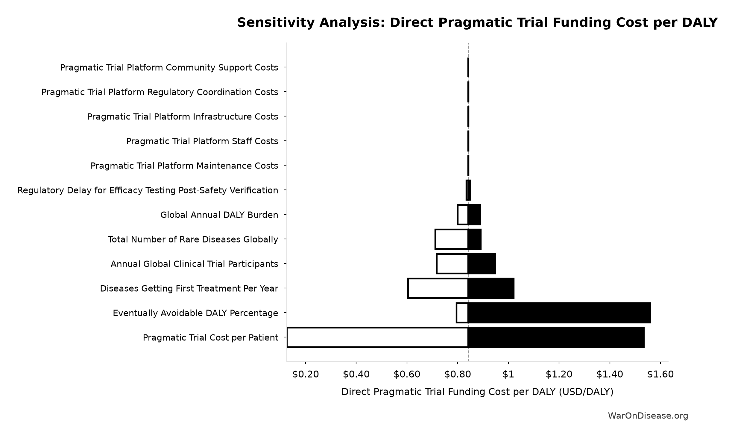
Sensitivity Indices for Direct Pragmatic Trial Funding Cost per DALY
Regression-based sensitivity showing which inputs explain the most variance in the output.
| Input Parameter | Sensitivity Coefficient | Interpretation |
|---|---|---|
| Direct Pragmatic Trial Funding NPV (Exploration Period) (USD) | 0.7920 | Strong driver |
| Total DALYs from Elimination of Efficacy Lag Plus Earlier Treatment Discovery from Higher Trial Throughput (DALYs) | -0.7046 | Strong driver |
Interpretation: Standardized coefficients show the change in output (in SD units) per 1 SD change in input. Values near ±1 indicate strong influence; values exceeding ±1 may occur with correlated inputs.
Monte Carlo Distribution
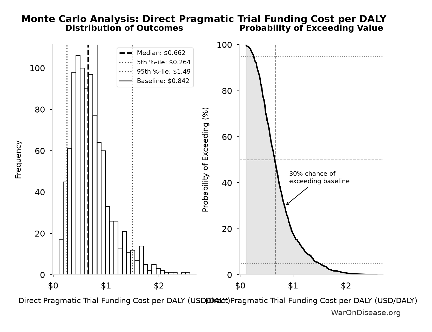
Simulation Results Summary: Direct Pragmatic Trial Funding Cost per DALY
| Statistic | Value |
|---|---|
| Baseline (deterministic) | $0.842 |
| Mean (expected value) | $0.742 |
| Median (50th percentile) | $0.662 |
| Standard Deviation | $0.395 |
| 90% Range (5th-95th percentile) | [$0.264, $1.49] |
The histogram shows 1,000 of the 10,000 Monte Carlo draws for Direct Pragmatic Trial Funding Cost per DALY; the summary statistics use all 10,000. The exceedance curve (right) shows the probability of the outcome exceeding any given value.
Exceedance Probability
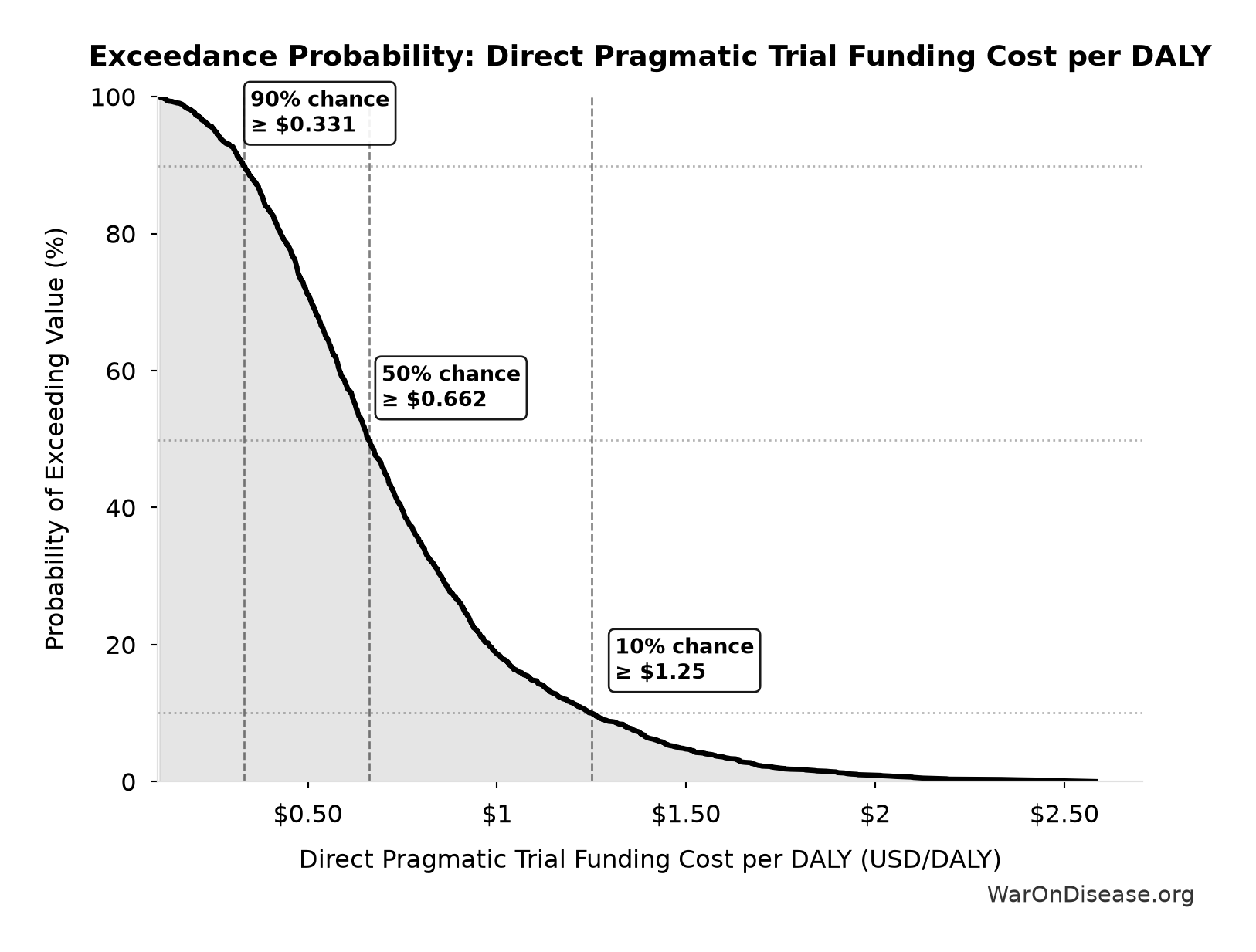
This exceedance probability chart shows the likelihood that Direct Pragmatic Trial Funding Cost per DALY will exceed any given threshold. The higher the curve at a threshold, the more likely the value exceeds it.
Direct Pragmatic Trial Funding NPV (Exploration Period): $476 billion
Note📊 Details
NPV of annual direct funding for the therapeutic space exploration period. Funding period equals exploration time (queue clearance years at given capacity multiplier). After exploration completes, the full timeline shift benefit is realized.
Inputs:
- Reference Annual Pragmatic Trial Funding: $21.8 billion
- Standard Discount Rate for NPV Analysis: 3%
- Therapeutic Space Exploration Time at Treaty-Scale Trial Capacity 🔢: 36 years
\[ \begin{gathered} NPV_{direct} \\ = \frac{T_{queue,trial}}{Funding_{trial,ref} \times r_{discount}} \\ = \frac{36}{\$21.8B \times 3\%} \\ = \$476B \end{gathered} \] where: \[ \begin{gathered} T_{queue,trial} \\ = \frac{T_{queue,SQ}}{k_{capacity}} \\ = \frac{443}{12.3} \\ = 36 \end{gathered} \] where: \[ \begin{gathered} T_{queue,SQ} \\ = \frac{N_{untreated}}{Treatments_{new,ann}} \\ = \frac{6{,}650}{15} \\ = 443 \end{gathered} \] where: \[ \begin{gathered} N_{untreated} \\ = N_{rare} \times 0.95 \\ = 7{,}000 \times 0.95 \\ = 6{,}650 \end{gathered} \] where: \[ \begin{gathered} k_{capacity} \\ = \frac{N_{fundable,ref}}{Slots_{curr}} \\ = \frac{23.4M}{1.9M} \\ = 12.3 \end{gathered} \] where: \[ \begin{gathered} N_{fundable,ref} \\ = \frac{Subsidies_{trial,ref}}{Cost_{pragmatic,pt}} \\ = \frac{\$21.8B}{\$929} \\ = 23.4M \end{gathered} \] where: \[ \begin{gathered} Subsidies_{trial,ref} \\ = Funding_{trial,ref} - OPEX_{trial} \\ = \$21.8B - \$40M \\ = \$21.8B \end{gathered} \] where: \[ \begin{gathered} OPEX_{trial} \\ = Cost_{platform} + Cost_{staff} + Cost_{infra} \\ + Cost_{regulatory} + Cost_{community} \\ = \$15M + \$10M + \$8M + \$5M + \$2M \\ = \$40M \end{gathered} \] ✓ High confidence
Sensitivity Analysis
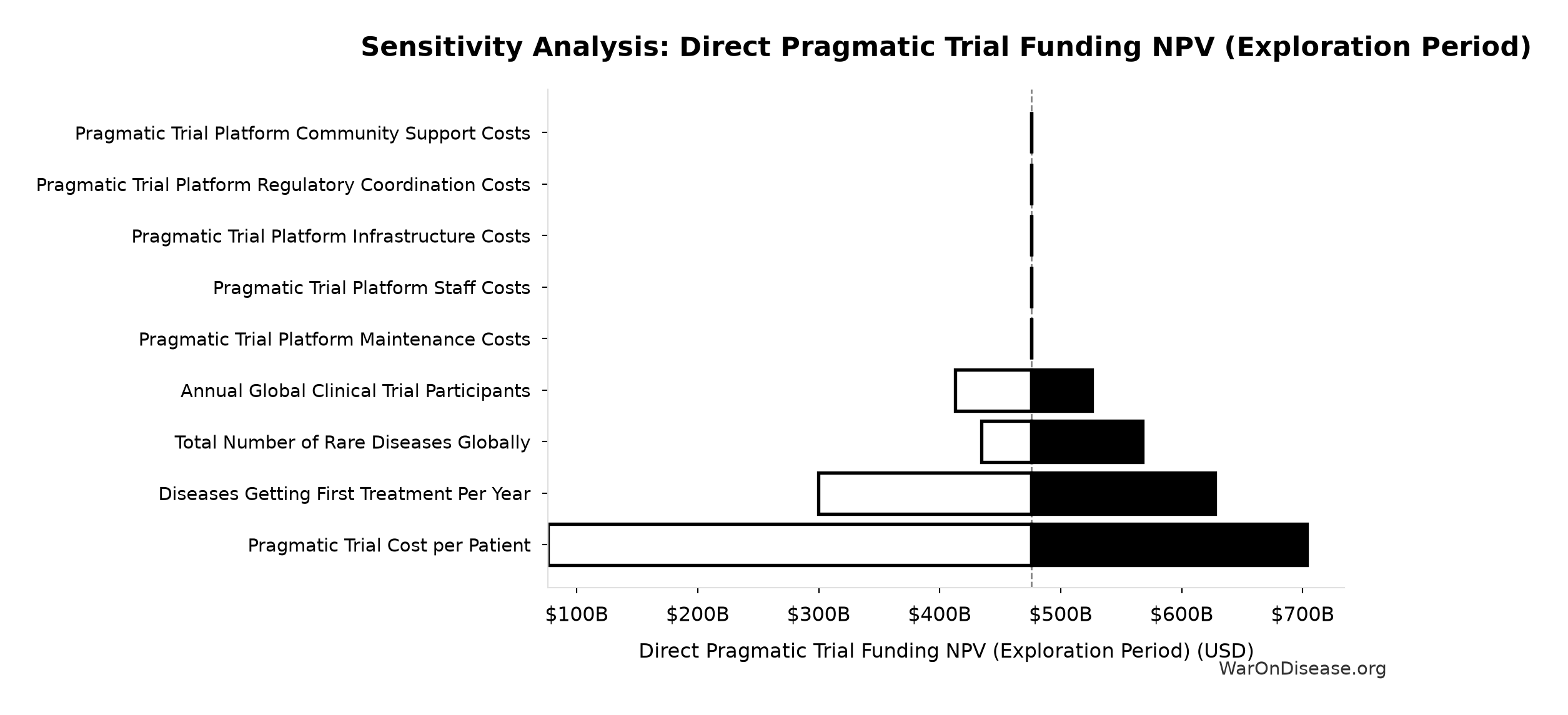
Sensitivity Indices for Direct Pragmatic Trial Funding NPV (Exploration Period)
Regression-based sensitivity showing which inputs explain the most variance in the output.
| Input Parameter | Sensitivity Coefficient | Interpretation |
|---|---|---|
| Therapeutic Space Exploration Time at Treaty-Scale Trial Capacity (years) | 0.8645 | Strong driver |
Interpretation: Standardized coefficients show the change in output (in SD units) per 1 SD change in input. Values near ±1 indicate strong influence; values exceeding ±1 may occur with correlated inputs.
Monte Carlo Distribution
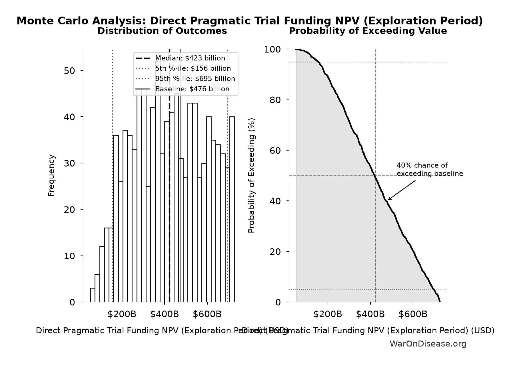
Simulation Results Summary: Direct Pragmatic Trial Funding NPV (Exploration Period)
| Statistic | Value |
|---|---|
| Baseline (deterministic) | $476 billion |
| Mean (expected value) | $425 billion |
| Median (50th percentile) | $423 billion |
| Standard Deviation | $169 billion |
| 90% Range (5th-95th percentile) | [$156 billion, $695 billion] |
The histogram shows 1,000 of the 10,000 Monte Carlo draws for Direct Pragmatic Trial Funding NPV (Exploration Period); the summary statistics use all 10,000. The exceedance curve (right) shows the probability of the outcome exceeding any given value.
Exceedance Probability
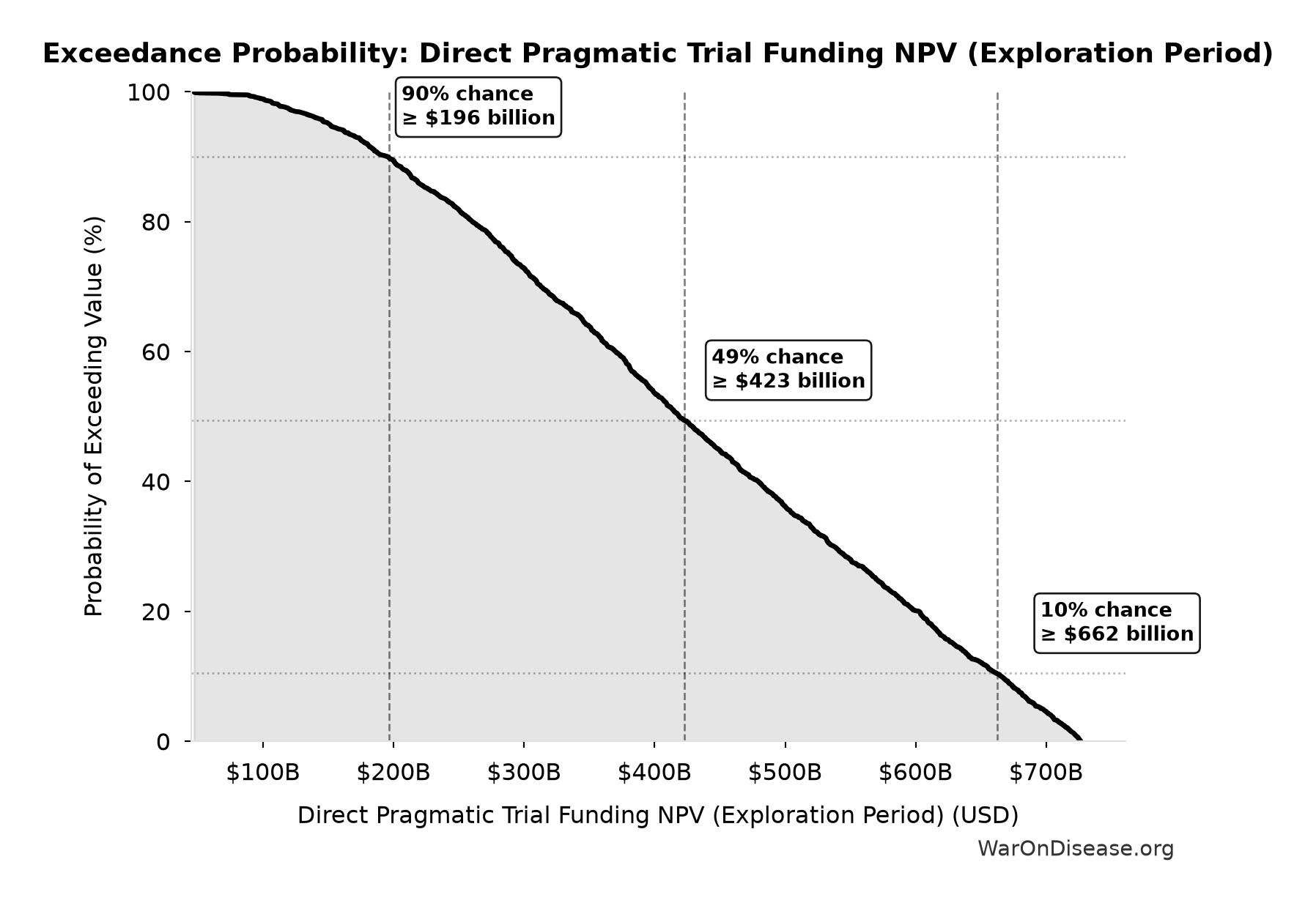
This exceedance probability chart shows the likelihood that Direct Pragmatic Trial Funding NPV (Exploration Period) will exceed any given threshold. The higher the curve at a threshold, the more likely the value exceeds it.
Direct Funding ROI - Elimination of Efficacy Lag Plus Earlier Treatment Discovery from Increased Trial Throughput: 178 thousand:1
Note📊 Details
ROI from directly funding pragmatic clinical trials over the therapeutic space exploration period.
Inputs:
- Total Economic Benefit from Elimination of Efficacy Lag Plus Earlier Treatment Discovery from Higher Trial Throughput 🔢: $84.8 quadrillion
- Direct Pragmatic Trial Funding NPV (Exploration Period) 🔢: $476 billion
\[ \begin{gathered} ROI_{direct,max} \\ = \frac{Value_{max}}{NPV_{direct}} \\ = \frac{\$84800T}{\$476B} \\ = 178{,}000 \end{gathered} \] where: \[ \begin{gathered} Value_{max} \\ = DALYs_{max} \times Value_{QALY} \\ = 565B \times \$150K \\ = \$84800T \end{gathered} \] where: \[ \begin{gathered} DALYs_{max} \\ = DALYs_{global,ann} \times Pct_{avoid,DALY} \times T_{accel,max} \\ = 2.88B \times 92.6\% \times 212 \\ = 565B \end{gathered} \] where: \[ T_{accel,max} = T_{accel} + T_{lag} = 204 + 8.2 = 212 \] where: \[ \begin{gathered} T_{accel} \\ = T_{first,SQ} \times \left(1 - \frac{1}{k_{capacity}}\right) \\ = 222 \times \left(1 - \frac{1}{12.3}\right) \\ = 204 \end{gathered} \] where: \[ \begin{gathered} T_{first,SQ} \\ = T_{queue,SQ} \times 0.5 \\ = 443 \times 0.5 \\ = 222 \end{gathered} \] where: \[ \begin{gathered} T_{queue,SQ} \\ = \frac{N_{untreated}}{Treatments_{new,ann}} \\ = \frac{6{,}650}{15} \\ = 443 \end{gathered} \] where: \[ \begin{gathered} N_{untreated} \\ = N_{rare} \times 0.95 \\ = 7{,}000 \times 0.95 \\ = 6{,}650 \end{gathered} \] where: \[ \begin{gathered} k_{capacity} \\ = \frac{N_{fundable,ref}}{Slots_{curr}} \\ = \frac{23.4M}{1.9M} \\ = 12.3 \end{gathered} \] where: \[ \begin{gathered} N_{fundable,ref} \\ = \frac{Subsidies_{trial,ref}}{Cost_{pragmatic,pt}} \\ = \frac{\$21.8B}{\$929} \\ = 23.4M \end{gathered} \] where: \[ \begin{gathered} Subsidies_{trial,ref} \\ = Funding_{trial,ref} - OPEX_{trial} \\ = \$21.8B - \$40M \\ = \$21.8B \end{gathered} \] where: \[ \begin{gathered} OPEX_{trial} \\ = Cost_{platform} + Cost_{staff} + Cost_{infra} \\ + Cost_{regulatory} + Cost_{community} \\ = \$15M + \$10M + \$8M + \$5M + \$2M \\ = \$40M \end{gathered} \] where: \[ \begin{gathered} NPV_{direct} \\ = \frac{T_{queue,trial}}{Funding_{trial,ref} \times r_{discount}} \\ = \frac{36}{\$21.8B \times 3\%} \\ = \$476B \end{gathered} \] where: \[ \begin{gathered} T_{queue,trial} \\ = \frac{T_{queue,SQ}}{k_{capacity}} \\ = \frac{443}{12.3} \\ = 36 \end{gathered} \] ✓ High confidence
Sensitivity Analysis
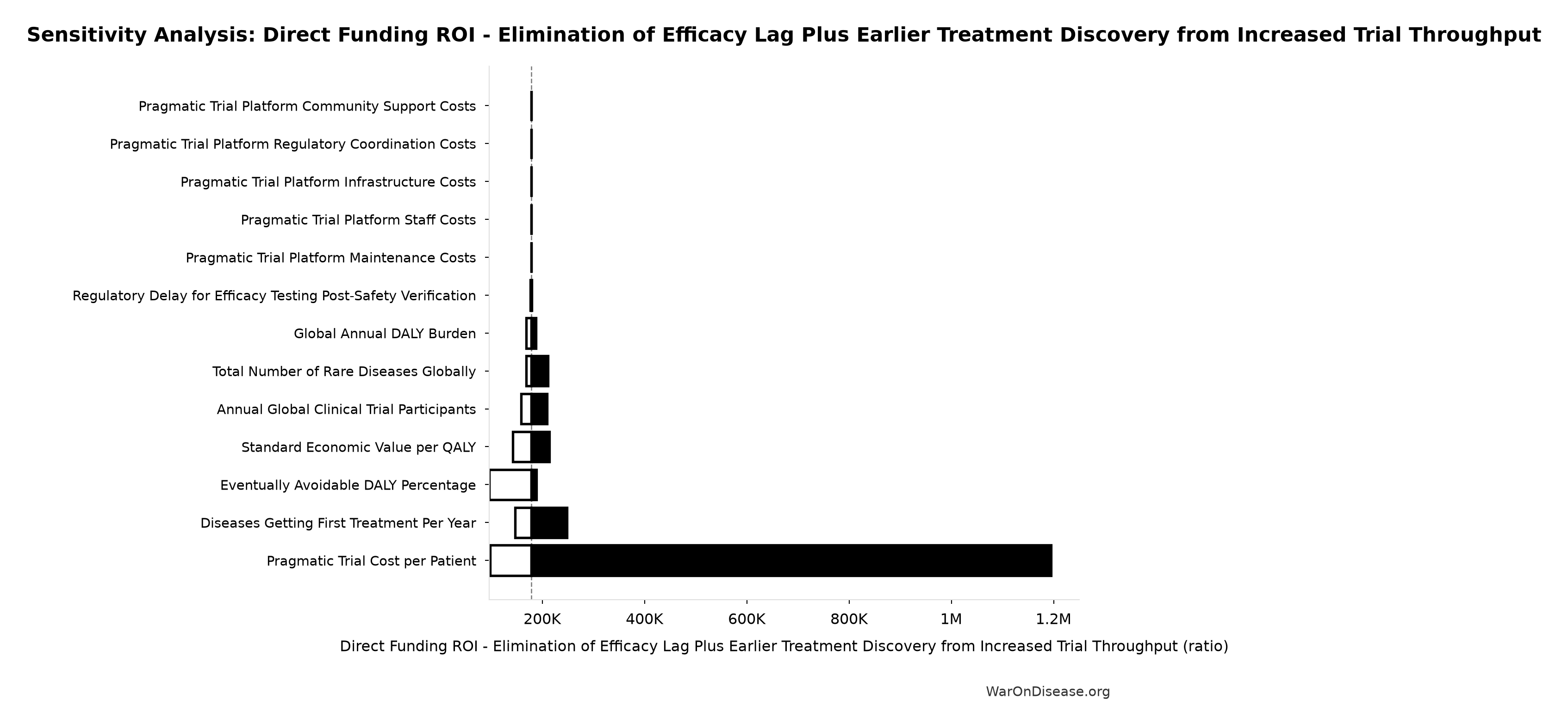
Sensitivity Indices for Direct Funding ROI - Elimination of Efficacy Lag Plus Earlier Treatment Discovery from Increased Trial Throughput
Regression-based sensitivity showing which inputs explain the most variance in the output.
| Input Parameter | Sensitivity Coefficient | Interpretation |
|---|---|---|
| Direct Pragmatic Trial Funding NPV (Exploration Period) (USD) | -0.7627 | Strong driver |
| Total Economic Benefit from Elimination of Efficacy Lag Plus Earlier Treatment Discovery from Higher Trial Throughput (USD) | 0.6139 | Strong driver |
Interpretation: Standardized coefficients show the change in output (in SD units) per 1 SD change in input. Values near ±1 indicate strong influence; values exceeding ±1 may occur with correlated inputs.
Monte Carlo Distribution
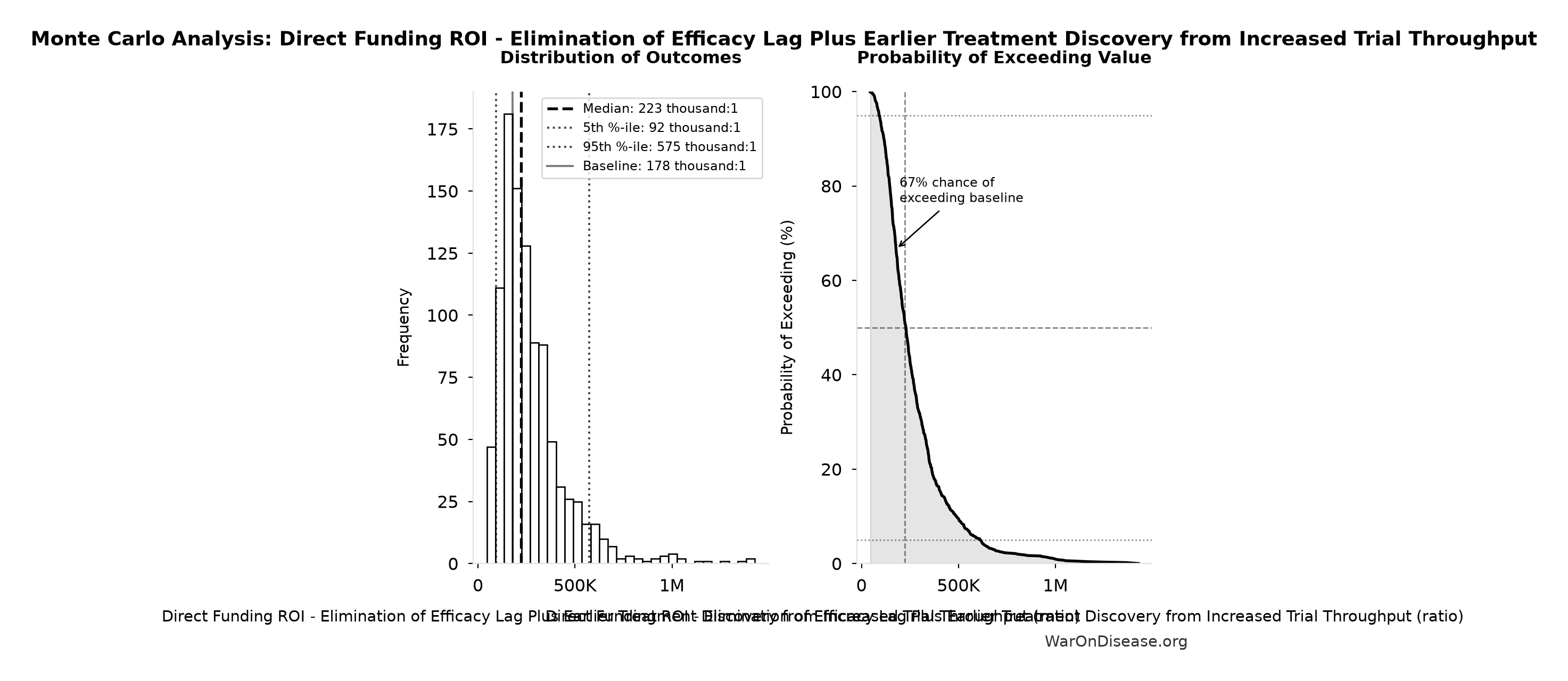
Simulation Results Summary: Direct Funding ROI - Elimination of Efficacy Lag Plus Earlier Treatment Discovery from Increased Trial Throughput
| Statistic | Value |
|---|---|
| Baseline (deterministic) | 178 thousand:1 |
| Mean (expected value) | 265 thousand:1 |
| Median (50th percentile) | 223 thousand:1 |
| Standard Deviation | 168 thousand:1 |
| 90% Range (5th-95th percentile) | [92 thousand:1, 575 thousand:1] |
The histogram shows 1,000 of the 10,000 Monte Carlo draws for Direct Funding ROI - Elimination of Efficacy Lag Plus Earlier Treatment Discovery from Increased Trial Throughput; the summary statistics use all 10,000. The exceedance curve (right) shows the probability of the outcome exceeding any given value.
Exceedance Probability
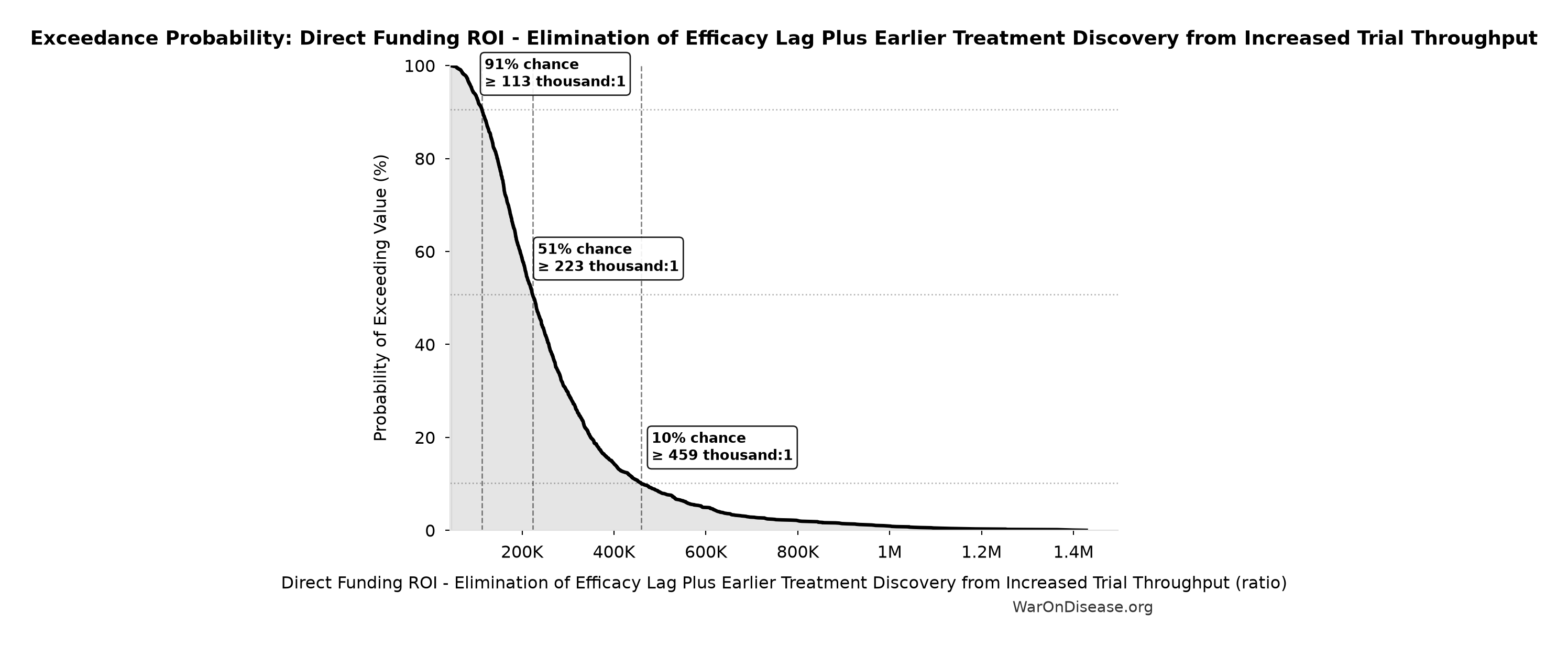
This exceedance probability chart shows the likelihood that Direct Funding ROI - Elimination of Efficacy Lag Plus Earlier Treatment Discovery from Increased Trial Throughput will exceed any given threshold. The higher the curve at a threshold, the more likely the value exceeds it.
Total DALYs Lost from Disease Eradication Delay: 8.77 billion DALYs
Note📊 Details
Total Disability-Adjusted Life Years lost from disease eradication delay (PRIMARY estimate)
Inputs:
- Years of Life Lost from Disease Eradication Delay 🔢: 7.9 billion years
- Years Lived with Disability During Disease Eradication Delay 🔢: 873 million years
\[ DALYs_{lag} = YLL_{lag} + YLD_{lag} = 7.9B + 873M = 8.77B \] where: \[ \begin{gathered} YLL_{lag} \\ = \text{DEATHS\_TOTAL} \times (REMAINING_LIFE_EXPECTANCY_AT_60 - (\text{MEAN\_AGE\_OF\_DEATH} - 60)) \end{gathered} \] where: \[ \begin{gathered} Deaths_{lag} \\ = T_{lag} \times Deaths_{disease,daily} \times 338 \\ = 8.2 \times 150{,}000 \times 338 \\ = 416M \end{gathered} \] where: \[ \begin{gathered} YLD_{lag} \\ = Deaths_{lag} \times T_{suffering} \times DW_{chronic} \\ = 416M \times 6 \times 0.35 \\ = 873M \end{gathered} \] ~ Medium confidence
Sensitivity Analysis
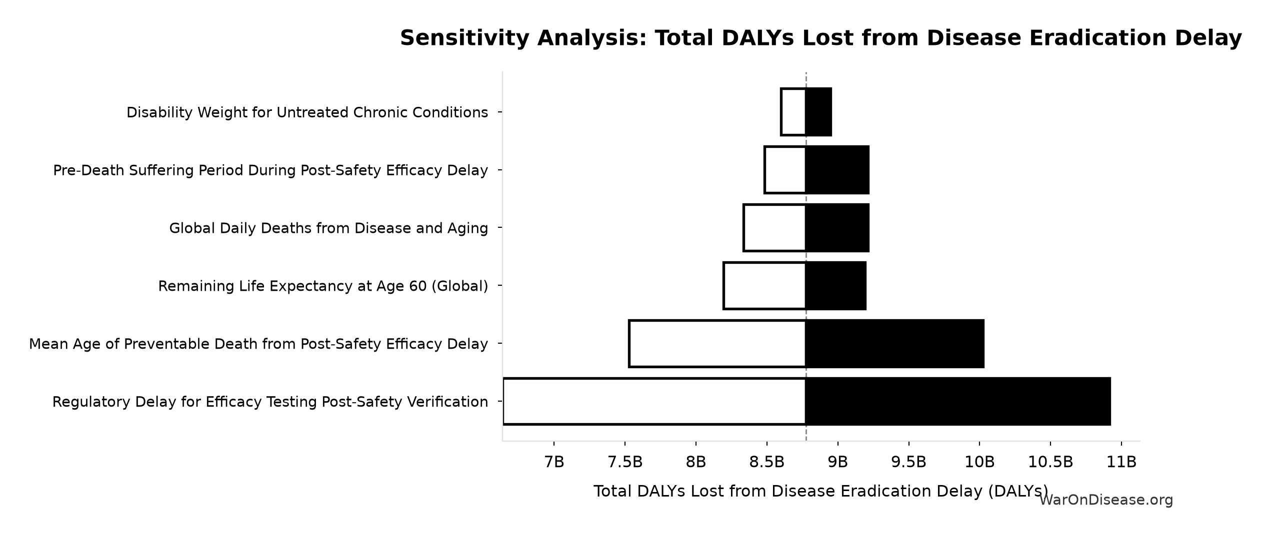
Sensitivity Indices for Total DALYs Lost from Disease Eradication Delay
Regression-based sensitivity showing which inputs explain the most variance in the output.
| Input Parameter | Sensitivity Coefficient | Interpretation |
|---|---|---|
| Years of Life Lost from Disease Eradication Delay (years) | 0.9243 | Strong driver |
| Years Lived with Disability During Disease Eradication Delay (years) | 0.1328 | Weak driver |
Interpretation: Standardized coefficients show the change in output (in SD units) per 1 SD change in input. Values near ±1 indicate strong influence; values exceeding ±1 may occur with correlated inputs.
Monte Carlo Distribution
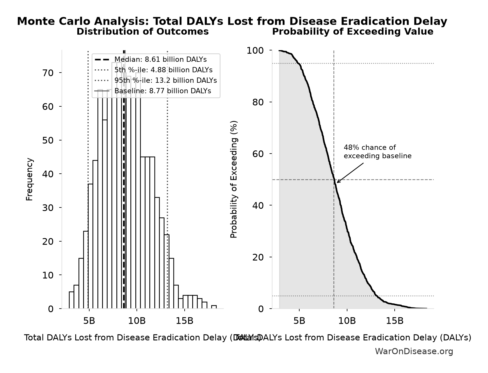
Simulation Results Summary: Total DALYs Lost from Disease Eradication Delay
| Statistic | Value |
|---|---|
| Baseline (deterministic) | 8.77 billion |
| Mean (expected value) | 8.78 billion |
| Median (50th percentile) | 8.61 billion |
| Standard Deviation | 2.55 billion |
| 90% Range (5th-95th percentile) | [4.88 billion, 13.2 billion] |
The histogram shows 1,000 of the 10,000 Monte Carlo draws for Total DALYs Lost from Disease Eradication Delay; the summary statistics use all 10,000. The exceedance curve (right) shows the probability of the outcome exceeding any given value.
Exceedance Probability
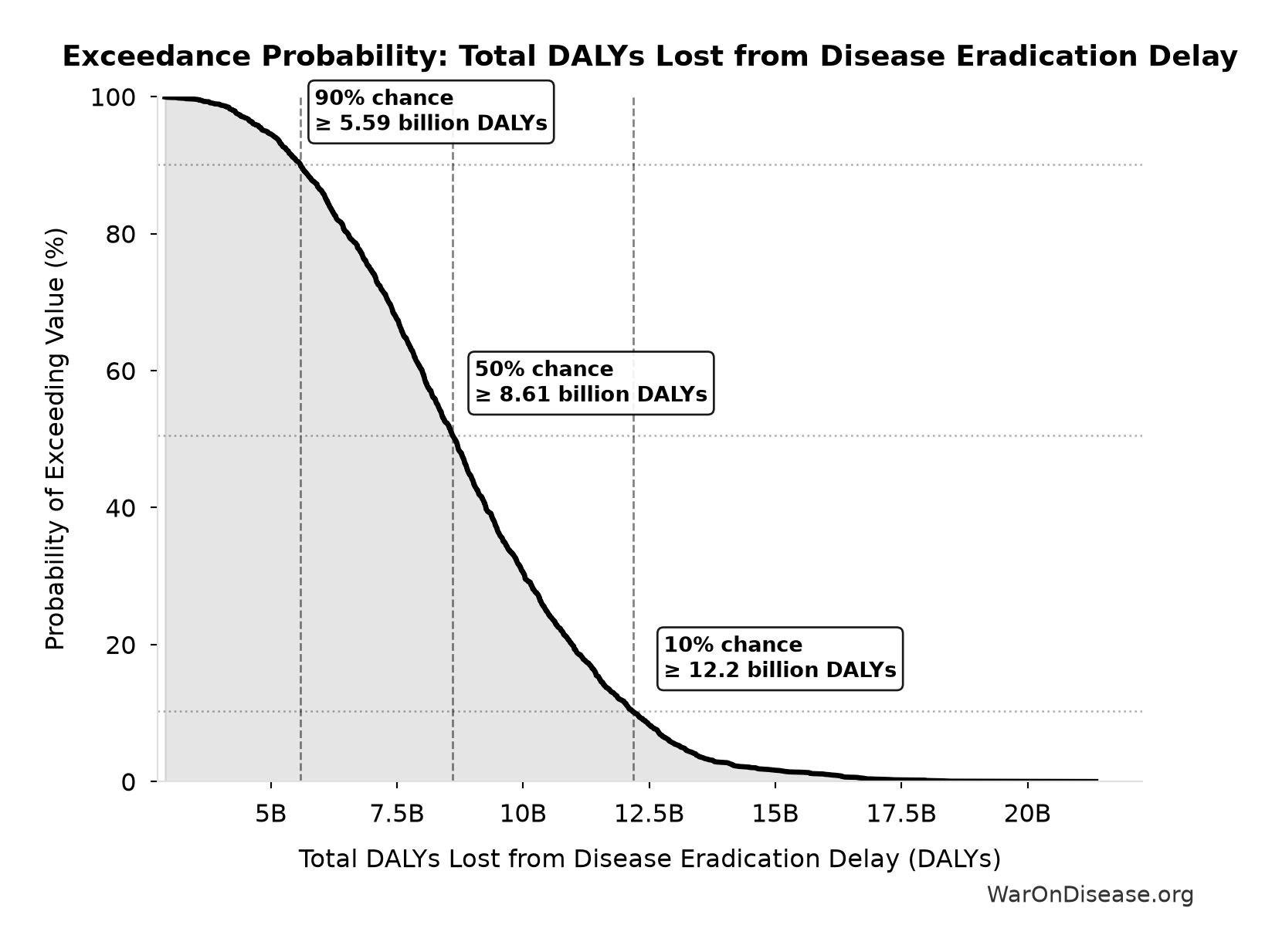
This exceedance probability chart shows the likelihood that Total DALYs Lost from Disease Eradication Delay will exceed any given threshold. The higher the curve at a threshold, the more likely the value exceeds it.
Total Deaths from Disease Eradication Delay: 416 million deaths
Note📊 Details
Total eventually avoidable deaths from delaying disease eradication by 8.2 years (PRIMARY estimate, conservative). Excludes fundamentally unavoidable deaths (primarily accidents ~7.9%).
Inputs:
- Regulatory Delay for Efficacy Testing Post-Safety Verification 📊: 8.2 years (SE: ±2 years)
- Global Daily Deaths from Disease and Aging 📊: 150 thousand deaths/day (SE: ±7,500 deaths/day)
\[ \begin{gathered} Deaths_{lag} \\ = T_{lag} \times Deaths_{disease,daily} \times 338 \\ = 8.2 \times 150{,}000 \times 338 \\ = 416M \end{gathered} \]
~ Medium confidence
Sensitivity Analysis
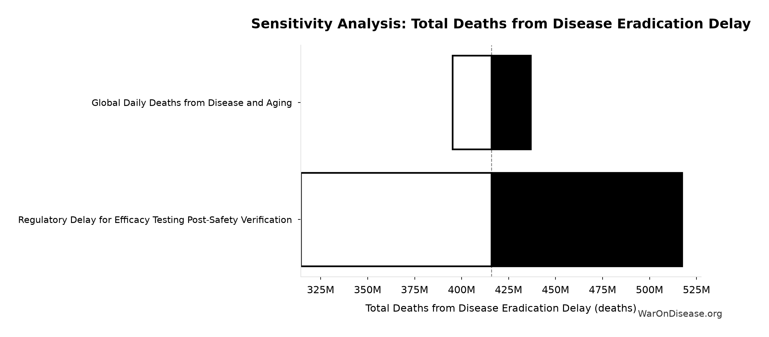
Sensitivity Indices for Total Deaths from Disease Eradication Delay
Regression-based sensitivity showing which inputs explain the most variance in the output.
| Input Parameter | Sensitivity Coefficient | Interpretation |
|---|---|---|
| Regulatory Delay for Efficacy Testing Post-Safety Verification (years) | 0.9809 | Strong driver |
| Global Daily Deaths from Disease and Aging (deaths/day) | 0.2015 | Weak driver |
Interpretation: Standardized coefficients show the change in output (in SD units) per 1 SD change in input. Values near ±1 indicate strong influence; values exceeding ±1 may occur with correlated inputs.
Monte Carlo Distribution
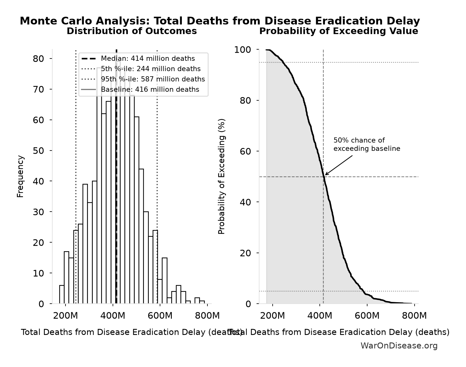
Simulation Results Summary: Total Deaths from Disease Eradication Delay
| Statistic | Value |
|---|---|
| Baseline (deterministic) | 416 million |
| Mean (expected value) | 416 million |
| Median (50th percentile) | 414 million |
| Standard Deviation | 103 million |
| 90% Range (5th-95th percentile) | [244 million, 587 million] |
The histogram shows 1,000 of the 10,000 Monte Carlo draws for Total Deaths from Disease Eradication Delay; the summary statistics use all 10,000. The exceedance curve (right) shows the probability of the outcome exceeding any given value.
Exceedance Probability
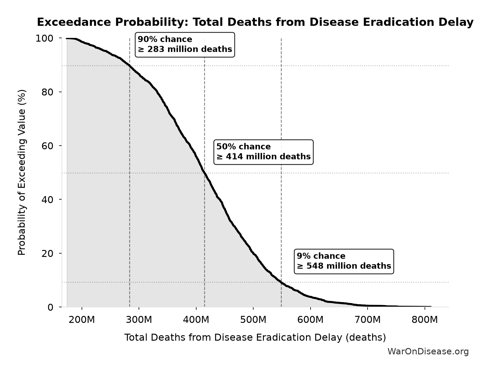
This exceedance probability chart shows the likelihood that Total Deaths from Disease Eradication Delay will exceed any given threshold. The higher the curve at a threshold, the more likely the value exceeds it.
Total Economic Loss from Disease Eradication Delay: $1.32 quadrillion
Note📊 Details
Total economic loss from delaying disease eradication by 8.2 years (PRIMARY estimate, 2024 USD). Values global DALYs at standardized US/International normative rate ($150k) rather than local ability-to-pay, representing the full human capital loss.
Inputs:
- Total DALYs Lost from Disease Eradication Delay 🔢: 8.77 billion DALYs
- Standard Economic Value per QALY 📊: $150,000 (SE: ±$30,000)
\[ \begin{gathered} Value_{lag} \\ = DALYs_{lag} \times Value_{QALY} \\ = 8.77B \times \$150K \\ = \$1320T \end{gathered} \] where: \[ DALYs_{lag} = YLL_{lag} + YLD_{lag} = 7.9B + 873M = 8.77B \] where: \[ \begin{gathered} YLL_{lag} \\ = \text{DEATHS\_TOTAL} \times (REMAINING_LIFE_EXPECTANCY_AT_60 - (\text{MEAN\_AGE\_OF\_DEATH} - 60)) \end{gathered} \] where: \[ \begin{gathered} Deaths_{lag} \\ = T_{lag} \times Deaths_{disease,daily} \times 338 \\ = 8.2 \times 150{,}000 \times 338 \\ = 416M \end{gathered} \] where: \[ \begin{gathered} YLD_{lag} \\ = Deaths_{lag} \times T_{suffering} \times DW_{chronic} \\ = 416M \times 6 \times 0.35 \\ = 873M \end{gathered} \] ~ Medium confidence
Sensitivity Analysis
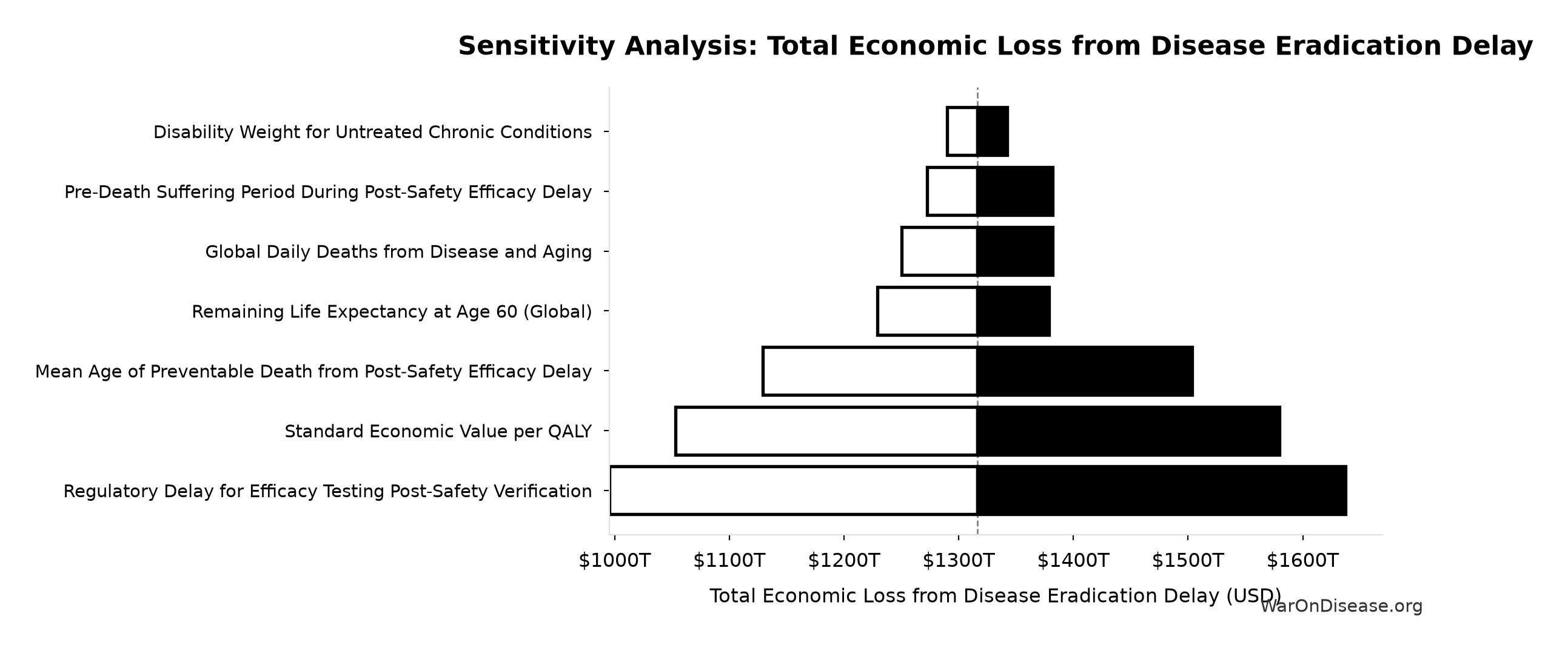
Sensitivity Indices for Total Economic Loss from Disease Eradication Delay
Regression-based sensitivity showing which inputs explain the most variance in the output.
| Input Parameter | Sensitivity Coefficient | Interpretation |
|---|---|---|
| Total DALYs Lost from Disease Eradication Delay (DALYs) | 0.8449 | Strong driver |
| Standard Economic Value per QALY (USD/QALY) | 0.5305 | Strong driver |
Interpretation: Standardized coefficients show the change in output (in SD units) per 1 SD change in input. Values near ±1 indicate strong influence; values exceeding ±1 may occur with correlated inputs.
Monte Carlo Distribution
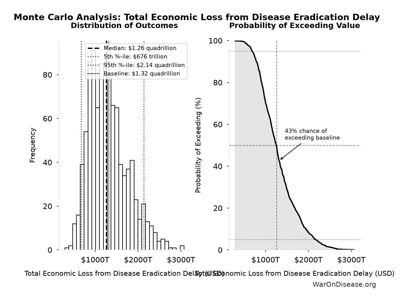
Simulation Results Summary: Total Economic Loss from Disease Eradication Delay
| Statistic | Value |
|---|---|
| Baseline (deterministic) | $1.32 quadrillion |
| Mean (expected value) | $1.31 quadrillion |
| Median (50th percentile) | $1.26 quadrillion |
| Standard Deviation | $452 trillion |
| 90% Range (5th-95th percentile) | [$676 trillion, $2.14 quadrillion] |
The histogram shows 1,000 of the 10,000 Monte Carlo draws for Total Economic Loss from Disease Eradication Delay; the summary statistics use all 10,000. The exceedance curve (right) shows the probability of the outcome exceeding any given value.
Exceedance Probability
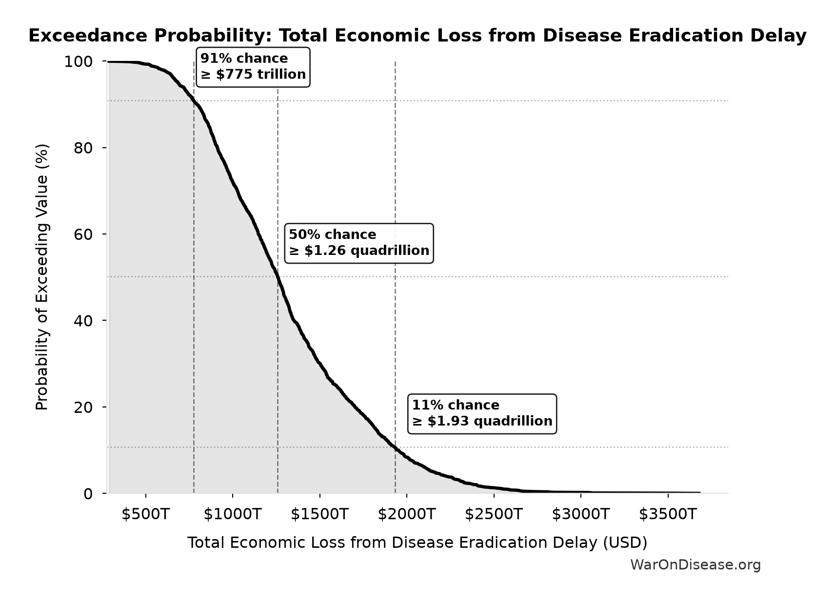
This exceedance probability chart shows the likelihood that Total Economic Loss from Disease Eradication Delay will exceed any given threshold. The higher the curve at a threshold, the more likely the value exceeds it.
Years Lived with Disability During Disease Eradication Delay: 873 million years
Note📊 Details
Years Lived with Disability during disease eradication delay (PRIMARY estimate)
Inputs:
- Total Deaths from Disease Eradication Delay 🔢: 416 million deaths
- Pre-Death Suffering Period During Post-Safety Efficacy Delay 📊: 6 years (95% CI: 4 years - 9 years)
- Disability Weight for Untreated Chronic Conditions 📊: 0.35 weight (SE: ±0.07 weight)
\[ \begin{gathered} YLD_{lag} \\ = Deaths_{lag} \times T_{suffering} \times DW_{chronic} \\ = 416M \times 6 \times 0.35 \\ = 873M \end{gathered} \] where: \[ \begin{gathered} Deaths_{lag} \\ = T_{lag} \times Deaths_{disease,daily} \times 338 \\ = 8.2 \times 150{,}000 \times 338 \\ = 416M \end{gathered} \] ~ Medium confidence
Sensitivity Analysis
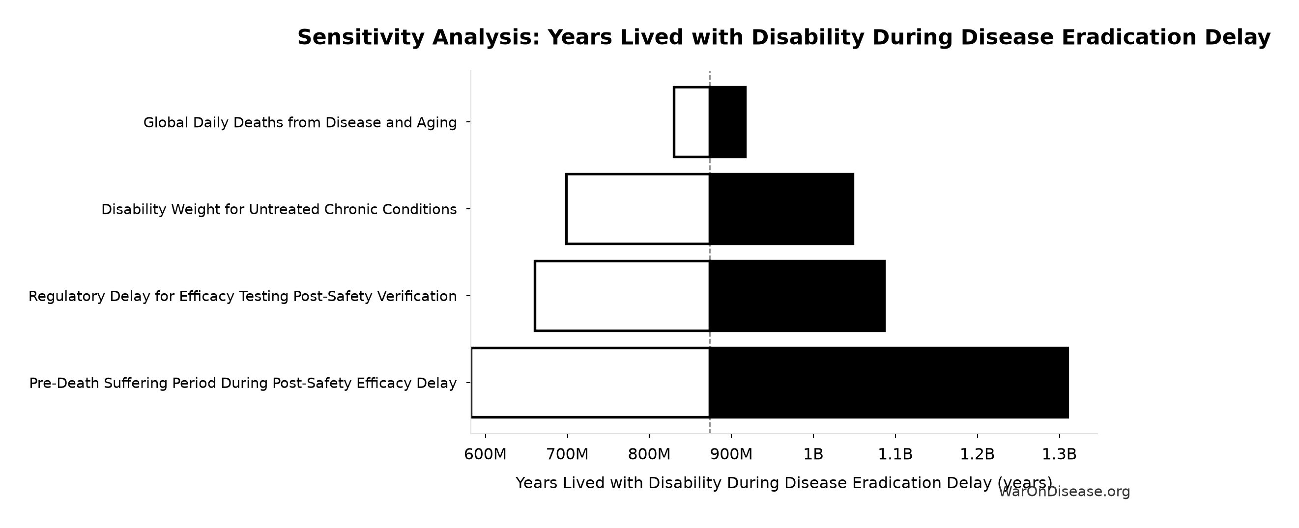
Sensitivity Indices for Years Lived with Disability During Disease Eradication Delay
Regression-based sensitivity showing which inputs explain the most variance in the output.
| Input Parameter | Sensitivity Coefficient | Interpretation |
|---|---|---|
| Total Deaths from Disease Eradication Delay (deaths) | 0.6338 | Strong driver |
| Pre-Death Suffering Period During Post-Safety Efficacy Delay (years) | 0.5588 | Strong driver |
| Disability Weight for Untreated Chronic Conditions (weight) | 0.5016 | Strong driver |
Interpretation: Standardized coefficients show the change in output (in SD units) per 1 SD change in input. Values near ±1 indicate strong influence; values exceeding ±1 may occur with correlated inputs.
Monte Carlo Distribution
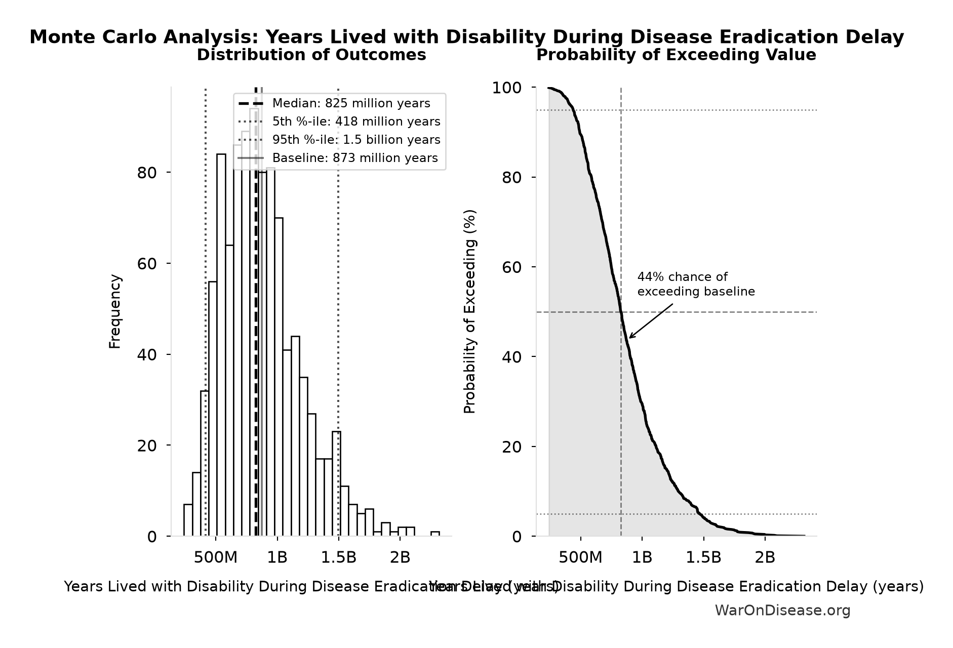
Simulation Results Summary: Years Lived with Disability During Disease Eradication Delay
| Statistic | Value |
|---|---|
| Baseline (deterministic) | 873 million |
| Mean (expected value) | 875 million |
| Median (50th percentile) | 825 million |
| Standard Deviation | 338 million |
| 90% Range (5th-95th percentile) | [418 million, 1.5 billion] |
The histogram shows 1,000 of the 10,000 Monte Carlo draws for Years Lived with Disability During Disease Eradication Delay; the summary statistics use all 10,000. The exceedance curve (right) shows the probability of the outcome exceeding any given value.
Exceedance Probability
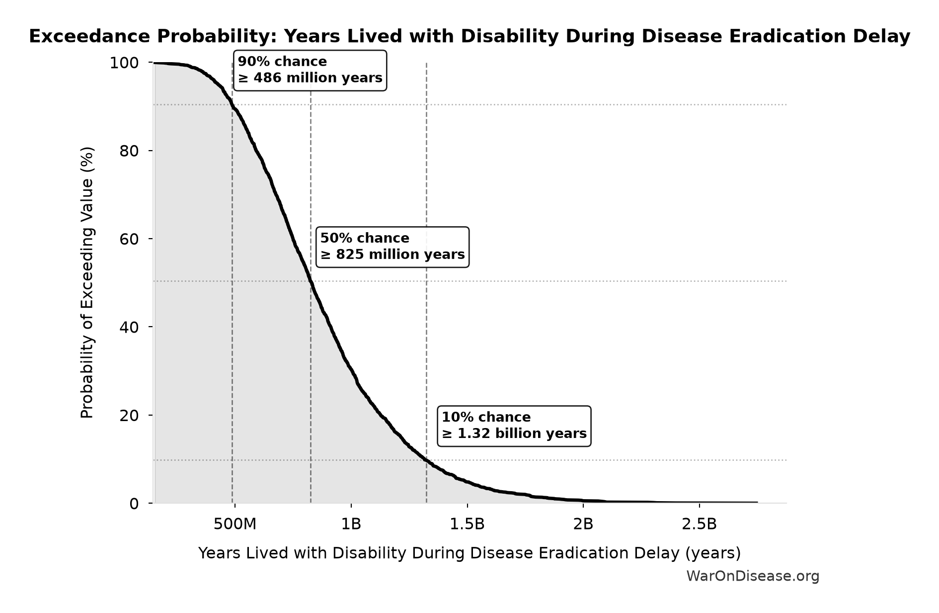
This exceedance probability chart shows the likelihood that Years Lived with Disability During Disease Eradication Delay will exceed any given threshold. The higher the curve at a threshold, the more likely the value exceeds it.
Years of Life Lost from Disease Eradication Delay: 7.9 billion years
Note📊 Details
Years of Life Lost from disease eradication delay deaths (PRIMARY estimate). Years lost per death = WHO conditional remaining life expectancy at 60, adjusted down to the mean lag-death age of 62 (~19 years/death). Replaces life-expectancy-at-birth minus age, which mixed an at-birth measure (carrying child mortality the deceased already survived) with a conditional question and understated the loss by ~40%. The linear age adjustment slightly understates remaining years (conditional life expectancy falls by less than one year per year of age).
Inputs:
- Total Deaths from Disease Eradication Delay 🔢: 416 million deaths
- Remaining Life Expectancy at Age 60 (Global) 📊: 21 years (95% CI: 19.6 years - 22 years)
- Mean Age of Preventable Death from Post-Safety Efficacy Delay 📊: 62 years (SE: ±3 years)
\[ \begin{gathered} YLL_{lag} \\ = \text{DEATHS\_TOTAL} \times (REMAINING_LIFE_EXPECTANCY_AT_60 - (\text{MEAN\_AGE\_OF\_DEATH} - 60)) \end{gathered} \] where: \[ \begin{gathered} Deaths_{lag} \\ = T_{lag} \times Deaths_{disease,daily} \times 338 \\ = 8.2 \times 150{,}000 \times 338 \\ = 416M \end{gathered} \] ~ Medium confidence
Sensitivity Analysis
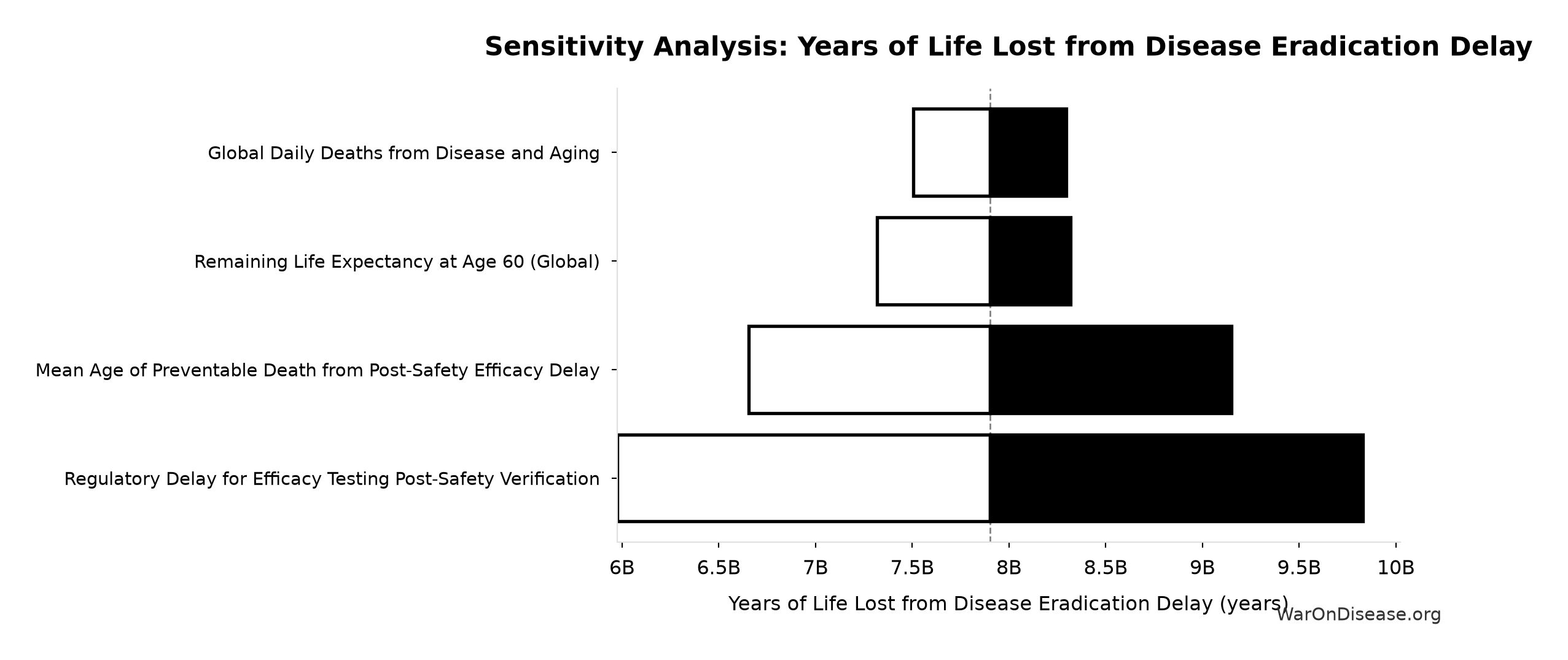
Sensitivity Indices for Years of Life Lost from Disease Eradication Delay
Regression-based sensitivity showing which inputs explain the most variance in the output.
| Input Parameter | Sensitivity Coefficient | Interpretation |
|---|---|---|
| Total Deaths from Disease Eradication Delay (deaths) | 0.8307 | Strong driver |
| Mean Age of Preventable Death from Post-Safety Efficacy Delay (years) | -0.5276 | Strong driver |
| Remaining Life Expectancy at Age 60 (Global) (years) | 0.1031 | Weak driver |
Interpretation: Standardized coefficients show the change in output (in SD units) per 1 SD change in input. Values near ±1 indicate strong influence; values exceeding ±1 may occur with correlated inputs.
Monte Carlo Distribution
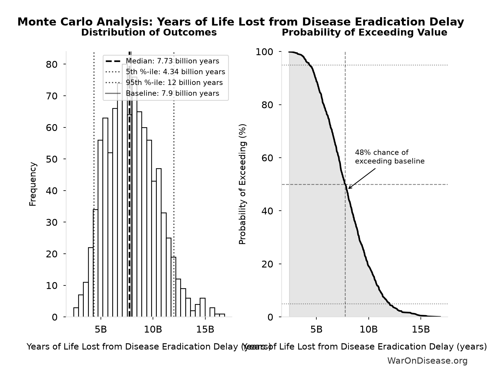
Simulation Results Summary: Years of Life Lost from Disease Eradication Delay
| Statistic | Value |
|---|---|
| Baseline (deterministic) | 7.9 billion |
| Mean (expected value) | 7.9 billion |
| Median (50th percentile) | 7.73 billion |
| Standard Deviation | 2.35 billion |
| 90% Range (5th-95th percentile) | [4.34 billion, 12 billion] |
The histogram shows 1,000 of the 10,000 Monte Carlo draws for Years of Life Lost from Disease Eradication Delay; the summary statistics use all 10,000. The exceedance curve (right) shows the probability of the outcome exceeding any given value.
Exceedance Probability
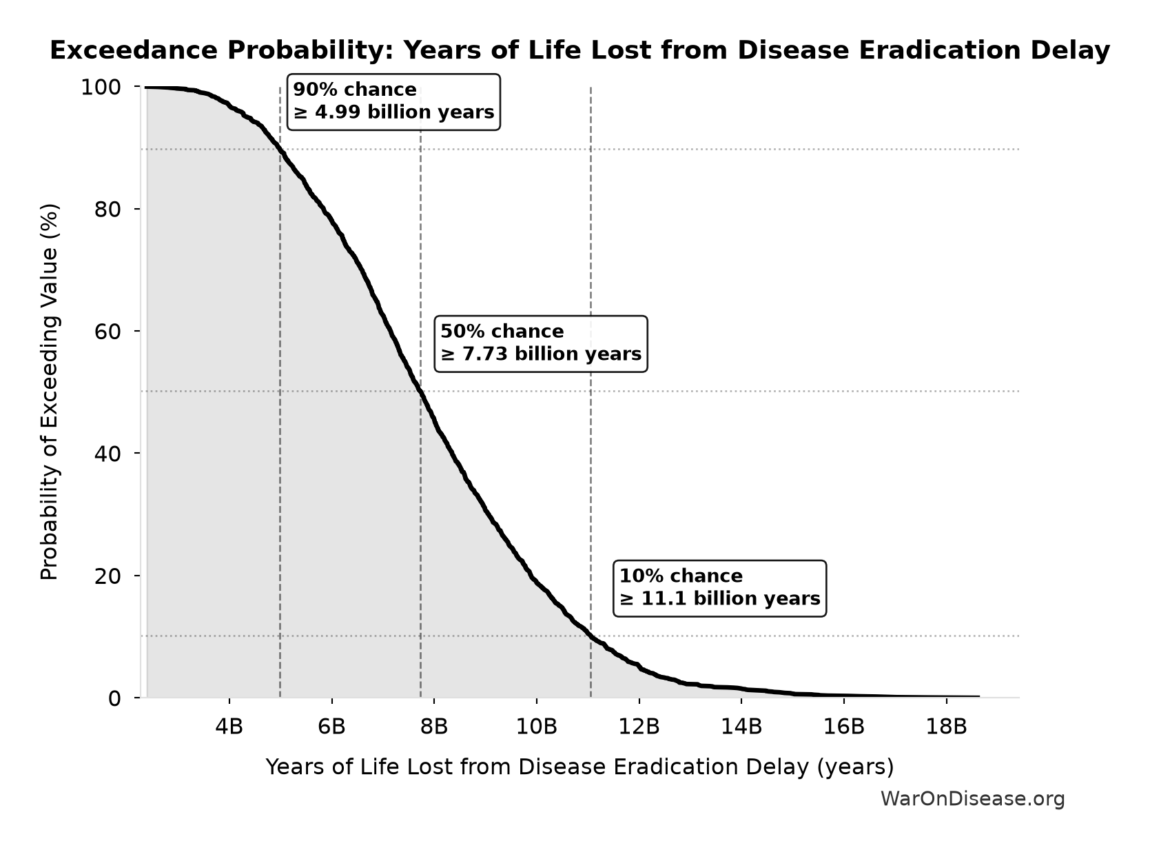
This exceedance probability chart shows the likelihood that Years of Life Lost from Disease Eradication Delay will exceed any given threshold. The higher the curve at a threshold, the more likely the value exceeds it.
New Treatments Per Year at Treaty-Scale Trial Capacity: 185 diseases/year
Note📊 Details
Diseases per year receiving their first effective treatment with treaty-scale pragmatic trial capacity. Scales proportionally with trial capacity multiplier.
Inputs:
- Diseases Getting First Treatment Per Year 📊: 15 diseases/year (95% CI: 8 diseases/year - 30 diseases/year)
- Pragmatic Trial Capacity Multiplier at Treaty-Scale Funding 🔢: 12.3x
\[ \begin{gathered} Treatments_{trial,ann} \\ = Treatments_{new,ann} \times k_{capacity} \\ = 15 \times 12.3 \\ = 185 \end{gathered} \] where: \[ \begin{gathered} k_{capacity} \\ = \frac{N_{fundable,ref}}{Slots_{curr}} \\ = \frac{23.4M}{1.9M} \\ = 12.3 \end{gathered} \] where: \[ \begin{gathered} N_{fundable,ref} \\ = \frac{Subsidies_{trial,ref}}{Cost_{pragmatic,pt}} \\ = \frac{\$21.8B}{\$929} \\ = 23.4M \end{gathered} \] where: \[ \begin{gathered} Subsidies_{trial,ref} \\ = Funding_{trial,ref} - OPEX_{trial} \\ = \$21.8B - \$40M \\ = \$21.8B \end{gathered} \] where: \[ \begin{gathered} OPEX_{trial} \\ = Cost_{platform} + Cost_{staff} + Cost_{infra} \\ + Cost_{regulatory} + Cost_{community} \\ = \$15M + \$10M + \$8M + \$5M + \$2M \\ = \$40M \end{gathered} \] ? Low confidence
Sensitivity Analysis
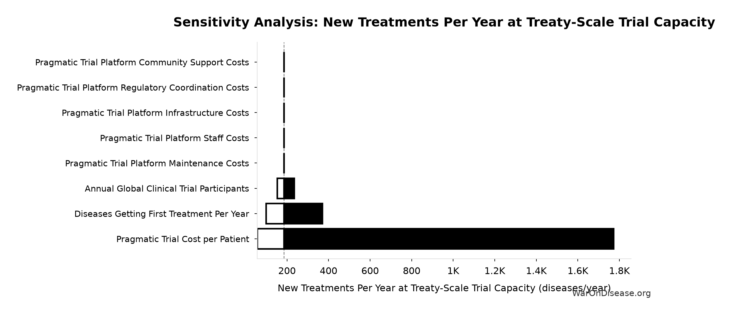
Sensitivity Indices for New Treatments Per Year at Treaty-Scale Trial Capacity
Regression-based sensitivity showing which inputs explain the most variance in the output.
| Input Parameter | Sensitivity Coefficient | Interpretation |
|---|---|---|
| Pragmatic Trial Capacity Multiplier at Treaty-Scale Funding (x) | 0.8722 | Strong driver |
| Diseases Getting First Treatment Per Year (diseases/year) | 0.3967 | Moderate driver |
Interpretation: Standardized coefficients show the change in output (in SD units) per 1 SD change in input. Values near ±1 indicate strong influence; values exceeding ±1 may occur with correlated inputs.
Monte Carlo Distribution
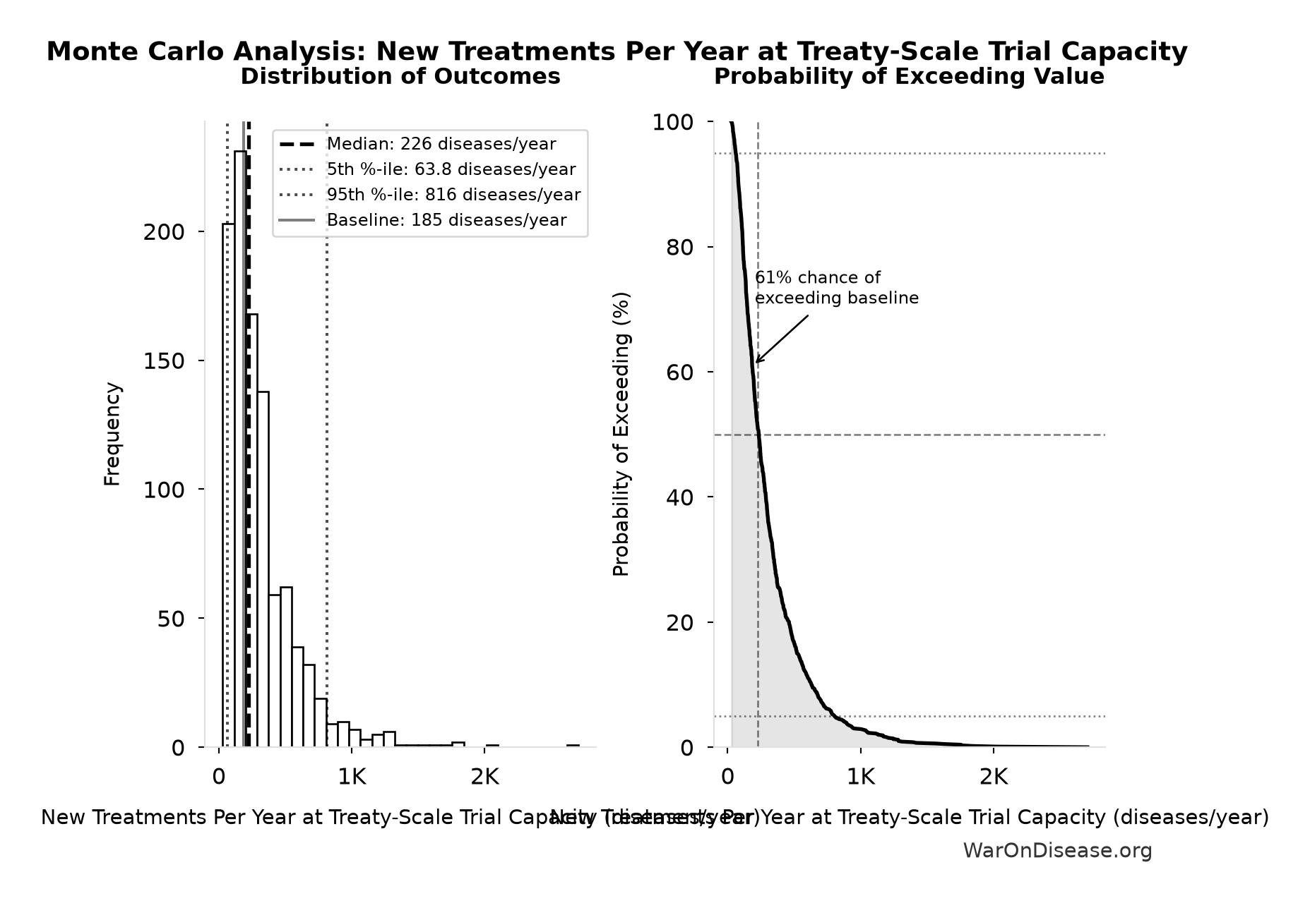
Simulation Results Summary: New Treatments Per Year at Treaty-Scale Trial Capacity
| Statistic | Value |
|---|---|
| Baseline (deterministic) | 185 |
| Mean (expected value) | 306 |
| Median (50th percentile) | 226 |
| Standard Deviation | 270 |
| 90% Range (5th-95th percentile) | [63.8, 816] |
The histogram shows 1,000 of the 10,000 Monte Carlo draws for New Treatments Per Year at Treaty-Scale Trial Capacity; the summary statistics use all 10,000. The exceedance curve (right) shows the probability of the outcome exceeding any given value.
Exceedance Probability
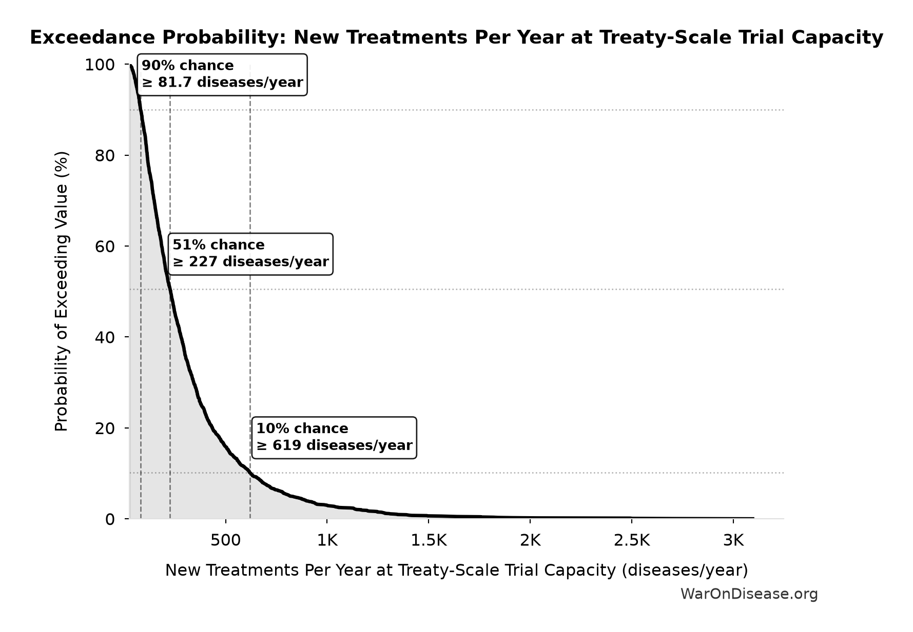
This exceedance probability chart shows the likelihood that New Treatments Per Year at Treaty-Scale Trial Capacity will exceed any given threshold. The higher the curve at a threshold, the more likely the value exceeds it.
Annual Net Savings from Pragmatic Trials (R&D Only): $40.4 billion
Note📊 Details
Annual net savings from R&D cost reduction only (gross savings minus operational costs, excludes regulatory delay value)
Inputs:
- Annual R&D Savings from Pragmatic Trials 🔢: $40.5 billion
- Total Annual Pragmatic Trial Platform Operational Costs 🔢: $40 million
\[ \begin{gathered} Savings_{RD,ann} \\ = Benefit_{RD,ann} - OPEX_{trial} \\ = \$40.5B - \$40M \\ = \$40.4B \end{gathered} \] where: \[ \begin{gathered} Benefit_{RD,ann} \\ = Spending_{trials} \times Pct_{P2+P3} \times Reduce_{pct} \\ = \$60B \times 69\% \times 97.7\% \\ = \$40.5B \end{gathered} \] where: \[ \begin{gathered} Reduce_{pct} \\ = 1 - \frac{Cost_{pragmatic,pt}}{Cost_{P3,pt}} \\ = 1 - \frac{\$929}{\$41K} \\ = 97.7\% \end{gathered} \] where: \[ \begin{gathered} OPEX_{trial} \\ = Cost_{platform} + Cost_{staff} + Cost_{infra} \\ + Cost_{regulatory} + Cost_{community} \\ = \$15M + \$10M + \$8M + \$5M + \$2M \\ = \$40M \end{gathered} \] ✓ High confidence
Sensitivity Analysis
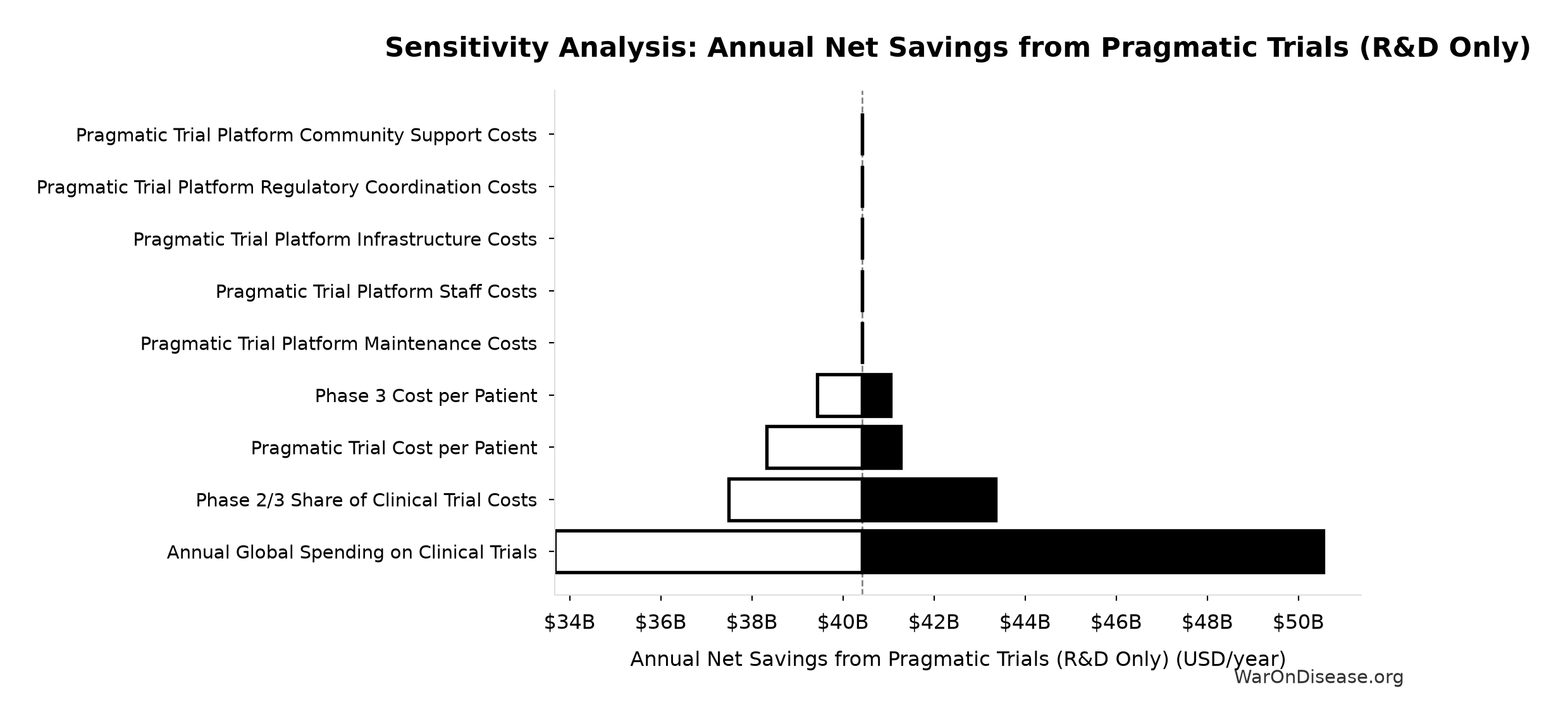
Sensitivity Indices for Annual Net Savings from Pragmatic Trials (R&D Only)
Regression-based sensitivity showing which inputs explain the most variance in the output.
| Input Parameter | Sensitivity Coefficient | Interpretation |
|---|---|---|
| Annual R&D Savings from Pragmatic Trials (USD/year) | 1.0000 | Strong driver |
| Total Annual Pragmatic Trial Platform Operational Costs (USD/year) | -0.0007 | Minimal effect |
Interpretation: Standardized coefficients show the change in output (in SD units) per 1 SD change in input. Values near ±1 indicate strong influence; values exceeding ±1 may occur with correlated inputs.
Monte Carlo Distribution
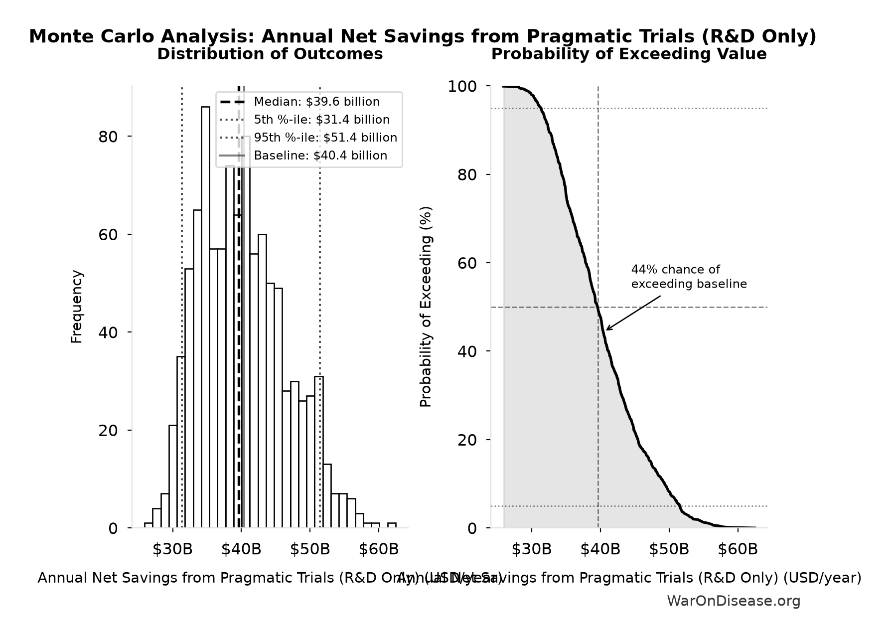
Simulation Results Summary: Annual Net Savings from Pragmatic Trials (R&D Only)
| Statistic | Value |
|---|---|
| Baseline (deterministic) | $40.4 billion |
| Mean (expected value) | $40.3 billion |
| Median (50th percentile) | $39.6 billion |
| Standard Deviation | $6.21 billion |
| 90% Range (5th-95th percentile) | [$31.4 billion, $51.4 billion] |
The histogram shows 1,000 of the 10,000 Monte Carlo draws for Annual Net Savings from Pragmatic Trials (R&D Only); the summary statistics use all 10,000. The exceedance curve (right) shows the probability of the outcome exceeding any given value.
Exceedance Probability
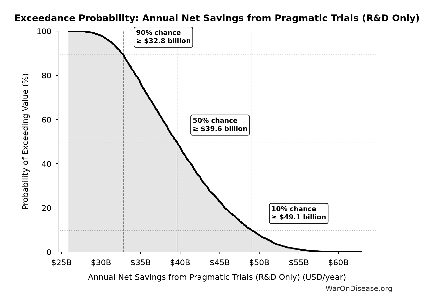
This exceedance probability chart shows the likelihood that Annual Net Savings from Pragmatic Trials (R&D Only) will exceed any given threshold. The higher the curve at a threshold, the more likely the value exceeds it.
Pragmatic Trial Platform Total NPV Annual OPEX: $40 million
Note📊 Details
Total NPV annual opex (pragmatic trial platform core + DIH initiatives)
Inputs:
- Pragmatic Trial Platform Core Framework Annual OPEX: $18.9 million (95% CI: $11 million - $26.5 million)
- DIH Broader Initiatives Annual OPEX: $21.1 million (95% CI: $14 million - $32 million)
\[ \begin{gathered} OPEX_{total} \\ = OPEX_{ann} + OPEX_{DIH,ann} \\ = \$18.9M + \$21.1M \\ = \$40M \end{gathered} \]
✓ High confidence
Sensitivity Analysis
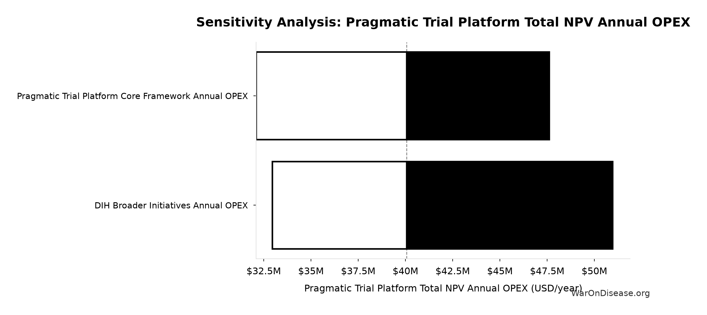
Sensitivity Indices for Pragmatic Trial Platform Total NPV Annual OPEX
Regression-based sensitivity showing which inputs explain the most variance in the output.
| Input Parameter | Sensitivity Coefficient | Interpretation |
|---|---|---|
| DIH Broader Initiatives Annual OPEX (USD/year) | 0.7686 | Strong driver |
| Pragmatic Trial Platform Core Framework Annual OPEX (USD/year) | 0.6508 | Strong driver |
Interpretation: Standardized coefficients show the change in output (in SD units) per 1 SD change in input. Values near ±1 indicate strong influence; values exceeding ±1 may occur with correlated inputs.
Monte Carlo Distribution
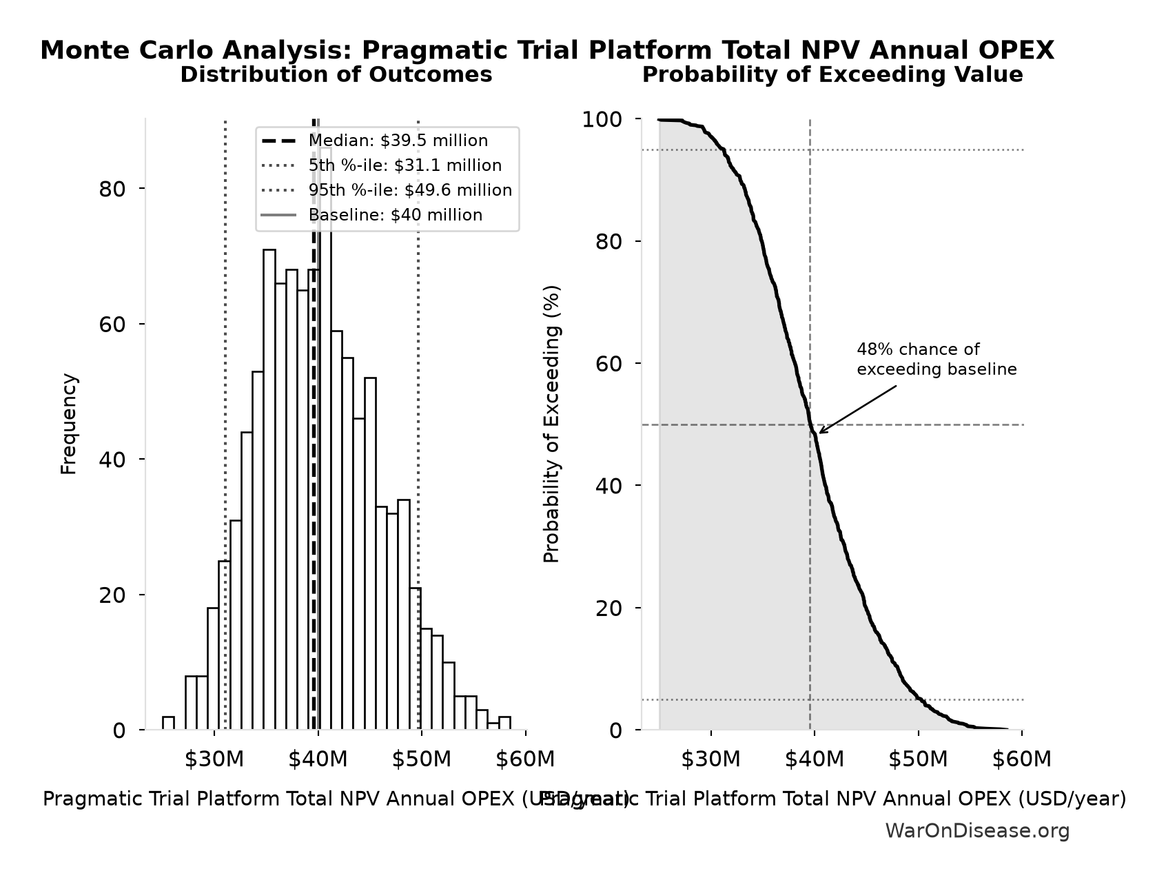
Simulation Results Summary: Pragmatic Trial Platform Total NPV Annual OPEX
| Statistic | Value |
|---|---|
| Baseline (deterministic) | $40 million |
| Mean (expected value) | $39.8 million |
| Median (50th percentile) | $39.5 million |
| Standard Deviation | $5.65 million |
| 90% Range (5th-95th percentile) | [$31.1 million, $49.6 million] |
The histogram shows 1,000 of the 10,000 Monte Carlo draws for Pragmatic Trial Platform Total NPV Annual OPEX; the summary statistics use all 10,000. The exceedance curve (right) shows the probability of the outcome exceeding any given value.
Exceedance Probability
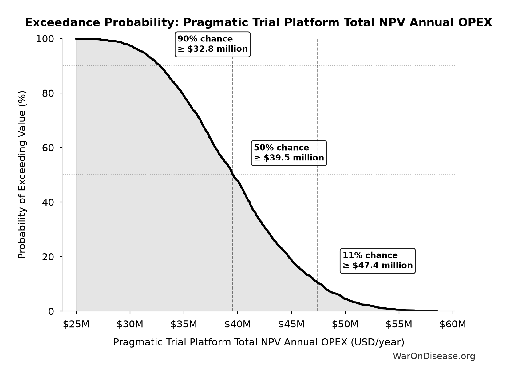
This exceedance probability chart shows the likelihood that Pragmatic Trial Platform Total NPV Annual OPEX will exceed any given threshold. The higher the curve at a threshold, the more likely the value exceeds it.
NPV of Pragmatic Trial Benefits (R&D Only, 10-Year Discounted): $269 billion
Note📊 Details
NPV of pragmatic trial R&D savings only with 5-year adoption ramp (10-year horizon, most conservative financial estimate)
Inputs:
- Annual Net Savings from Pragmatic Trials (R&D Only) 🔢: $40.4 billion
- Standard Discount Rate for NPV Analysis: 3%
\[ \begin{gathered} NPV_{RD} \\ = \sum_{t=1}^{10} \frac{Savings_{RD,ann} \cdot \frac{\min(t,5)}{5}}{(1+r)^t} \end{gathered} \]
✓ High confidence
Sensitivity Analysis
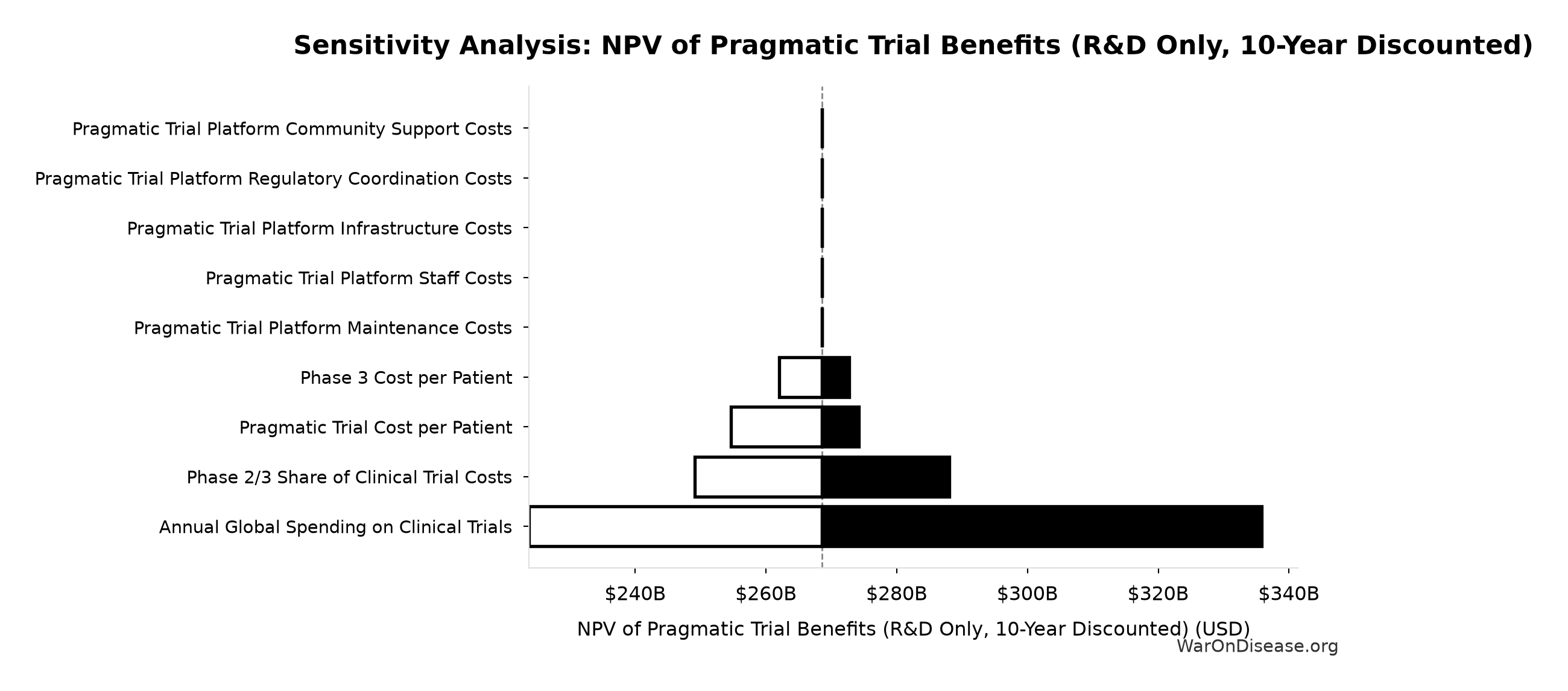
Sensitivity Indices for NPV of Pragmatic Trial Benefits (R&D Only, 10-Year Discounted)
Regression-based sensitivity showing which inputs explain the most variance in the output.
| Input Parameter | Sensitivity Coefficient | Interpretation |
|---|---|---|
| Annual Net Savings from Pragmatic Trials (R&D Only) (USD/year) | 1.0000 | Strong driver |
Interpretation: Standardized coefficients show the change in output (in SD units) per 1 SD change in input. Values near ±1 indicate strong influence; values exceeding ±1 may occur with correlated inputs.
Monte Carlo Distribution
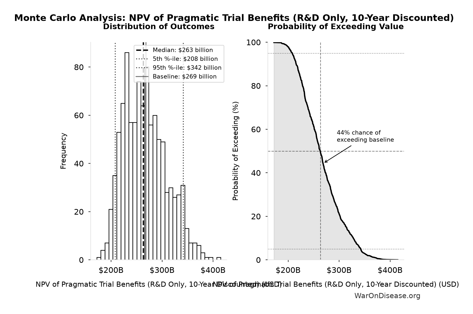
Simulation Results Summary: NPV of Pragmatic Trial Benefits (R&D Only, 10-Year Discounted)
| Statistic | Value |
|---|---|
| Baseline (deterministic) | $269 billion |
| Mean (expected value) | $268 billion |
| Median (50th percentile) | $263 billion |
| Standard Deviation | $41.3 billion |
| 90% Range (5th-95th percentile) | [$208 billion, $342 billion] |
The histogram shows 1,000 of the 10,000 Monte Carlo draws for NPV of Pragmatic Trial Benefits (R&D Only, 10-Year Discounted); the summary statistics use all 10,000. The exceedance curve (right) shows the probability of the outcome exceeding any given value.
Exceedance Probability
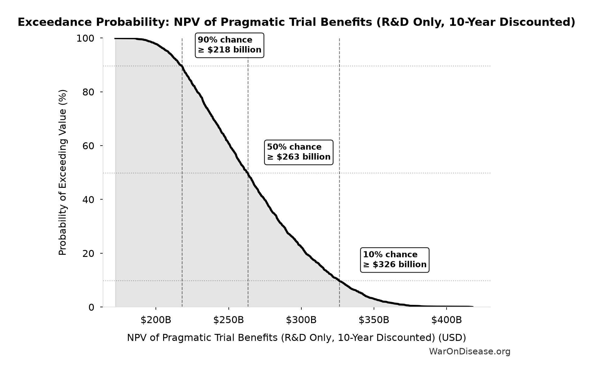
This exceedance probability chart shows the likelihood that NPV of Pragmatic Trial Benefits (R&D Only, 10-Year Discounted) will exceed any given threshold. The higher the curve at a threshold, the more likely the value exceeds it.
NPV Net Benefit (R&D Only): $268 billion
Note📊 Details
NPV net benefit using R&D savings only (benefits minus costs)
Inputs:
- NPV of Pragmatic Trial Benefits (R&D Only, 10-Year Discounted) 🔢: $269 billion
- Pragmatic Trial Platform Total NPV Cost 🔢: $611 million
\[ \begin{gathered} NPV_{net,RD} \\ = NPV_{RD} - Cost_{platform,total} \\ = \$269B - \$611M \\ = \$268B \end{gathered} \] where: \[ \begin{gathered} NPV_{RD} \\ = \sum_{t=1}^{10} \frac{Savings_{RD,ann} \cdot \frac{\min(t,5)}{5}}{(1+r)^t} \end{gathered} \] where: \[ \begin{gathered} Savings_{RD,ann} \\ = Benefit_{RD,ann} - OPEX_{trial} \\ = \$40.5B - \$40M \\ = \$40.4B \end{gathered} \] where: \[ \begin{gathered} Benefit_{RD,ann} \\ = Spending_{trials} \times Pct_{P2+P3} \times Reduce_{pct} \\ = \$60B \times 69\% \times 97.7\% \\ = \$40.5B \end{gathered} \] where: \[ \begin{gathered} Reduce_{pct} \\ = 1 - \frac{Cost_{pragmatic,pt}}{Cost_{P3,pt}} \\ = 1 - \frac{\$929}{\$41K} \\ = 97.7\% \end{gathered} \] where: \[ \begin{gathered} OPEX_{trial} \\ = Cost_{platform} + Cost_{staff} + Cost_{infra} \\ + Cost_{regulatory} + Cost_{community} \\ = \$15M + \$10M + \$8M + \$5M + \$2M \\ = \$40M \end{gathered} \] where: \[ \begin{gathered} Cost_{platform,total} \\ = PV_{OPEX} + Cost_{upfront,total} \\ = \$342M + \$270M \\ = \$611M \end{gathered} \] where: \[ \begin{gathered} PV_{OPEX} \\ = \frac{T_{horizon}}{OPEX_{total} \times r_{discount}} \\ = \frac{10}{\$40M \times 3\%} \\ = \$342M \end{gathered} \] where: \[ \begin{gathered} OPEX_{total} \\ = OPEX_{ann} + OPEX_{DIH,ann} \\ = \$18.9M + \$21.1M \\ = \$40M \end{gathered} \] where: \[ \begin{gathered} Cost_{upfront,total} \\ = Cost_{upfront} + Cost_{DIH,init} \\ = \$40M + \$230M \\ = \$270M \end{gathered} \] ✓ High confidence
Sensitivity Analysis
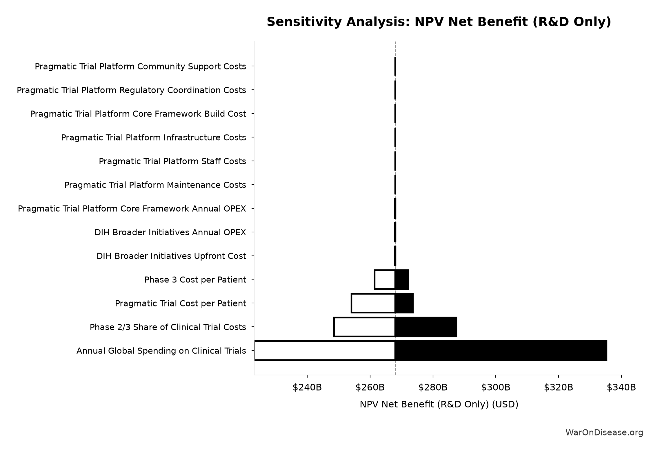
Sensitivity Indices for NPV Net Benefit (R&D Only)
Regression-based sensitivity showing which inputs explain the most variance in the output.
| Input Parameter | Sensitivity Coefficient | Interpretation |
|---|---|---|
| NPV of Pragmatic Trial Benefits (R&D Only, 10-Year Discounted) (USD) | 1.0000 | Strong driver |
| Pragmatic Trial Platform Total NPV Cost (USD) | -0.0017 | Minimal effect |
Interpretation: Standardized coefficients show the change in output (in SD units) per 1 SD change in input. Values near ±1 indicate strong influence; values exceeding ±1 may occur with correlated inputs.
Monte Carlo Distribution
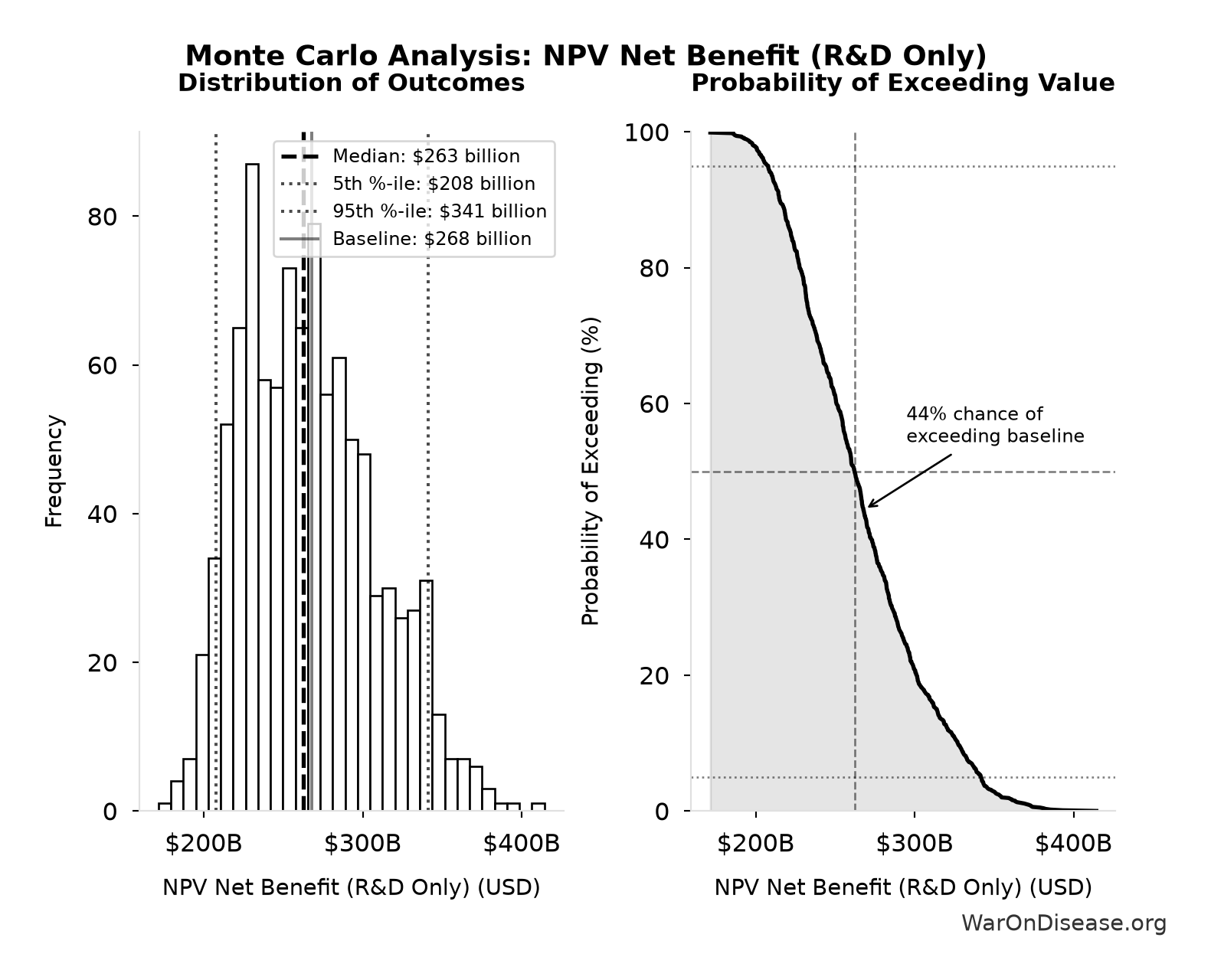
Simulation Results Summary: NPV Net Benefit (R&D Only)
| Statistic | Value |
|---|---|
| Baseline (deterministic) | $268 billion |
| Mean (expected value) | $267 billion |
| Median (50th percentile) | $263 billion |
| Standard Deviation | $41.3 billion |
| 90% Range (5th-95th percentile) | [$208 billion, $341 billion] |
The histogram shows 1,000 of the 10,000 Monte Carlo draws for NPV Net Benefit (R&D Only); the summary statistics use all 10,000. The exceedance curve (right) shows the probability of the outcome exceeding any given value.
Exceedance Probability
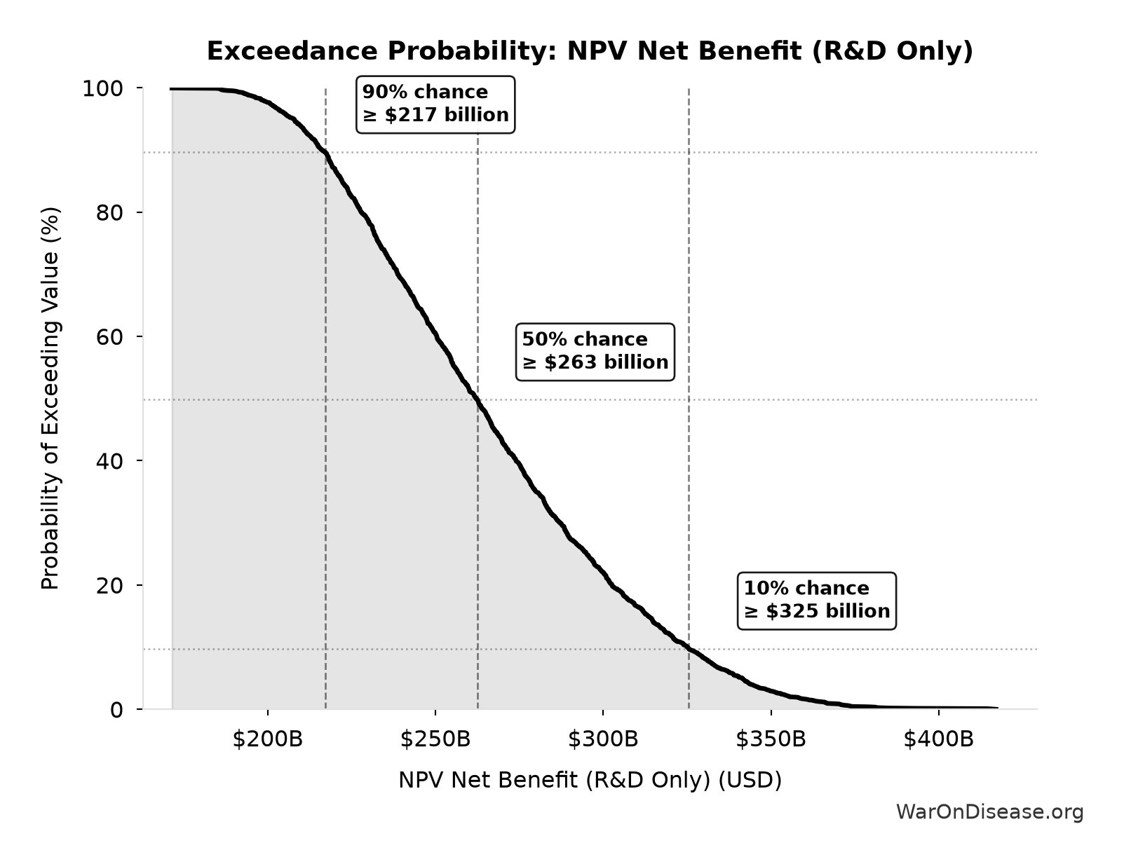
This exceedance probability chart shows the likelihood that NPV Net Benefit (R&D Only) will exceed any given threshold. The higher the curve at a threshold, the more likely the value exceeds it.
Pragmatic Trial Platform Present Value of Annual OPEX Over 10 Years: $342 million
Note📊 Details
Present value of annual opex over 10 years (NPV formula)
Inputs:
- Pragmatic Trial Platform Total NPV Annual OPEX 🔢: $40 million
- Standard Discount Rate for NPV Analysis: 3%
- Standard Time Horizon for NPV Analysis: 10 years
\[ \begin{gathered} PV_{OPEX} \\ = \frac{T_{horizon}}{OPEX_{total} \times r_{discount}} \\ = \frac{10}{\$40M \times 3\%} \\ = \$342M \end{gathered} \] where: \[ \begin{gathered} OPEX_{total} \\ = OPEX_{ann} + OPEX_{DIH,ann} \\ = \$18.9M + \$21.1M \\ = \$40M \end{gathered} \] ✓ High confidence
Sensitivity Analysis
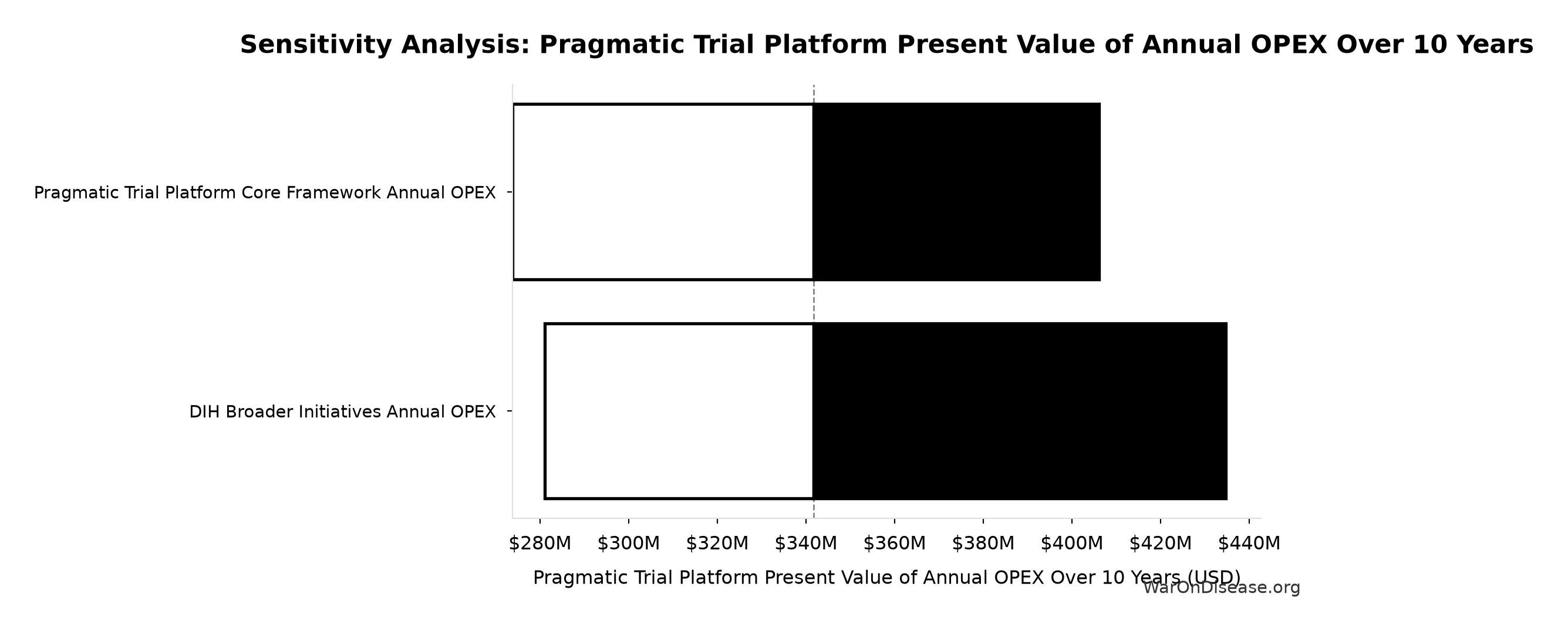
Sensitivity Indices for Pragmatic Trial Platform Present Value of Annual OPEX Over 10 Years
Regression-based sensitivity showing which inputs explain the most variance in the output.
| Input Parameter | Sensitivity Coefficient | Interpretation |
|---|---|---|
| Pragmatic Trial Platform Total NPV Annual OPEX (USD/year) | 1.0000 | Strong driver |
Interpretation: Standardized coefficients show the change in output (in SD units) per 1 SD change in input. Values near ±1 indicate strong influence; values exceeding ±1 may occur with correlated inputs.
Monte Carlo Distribution
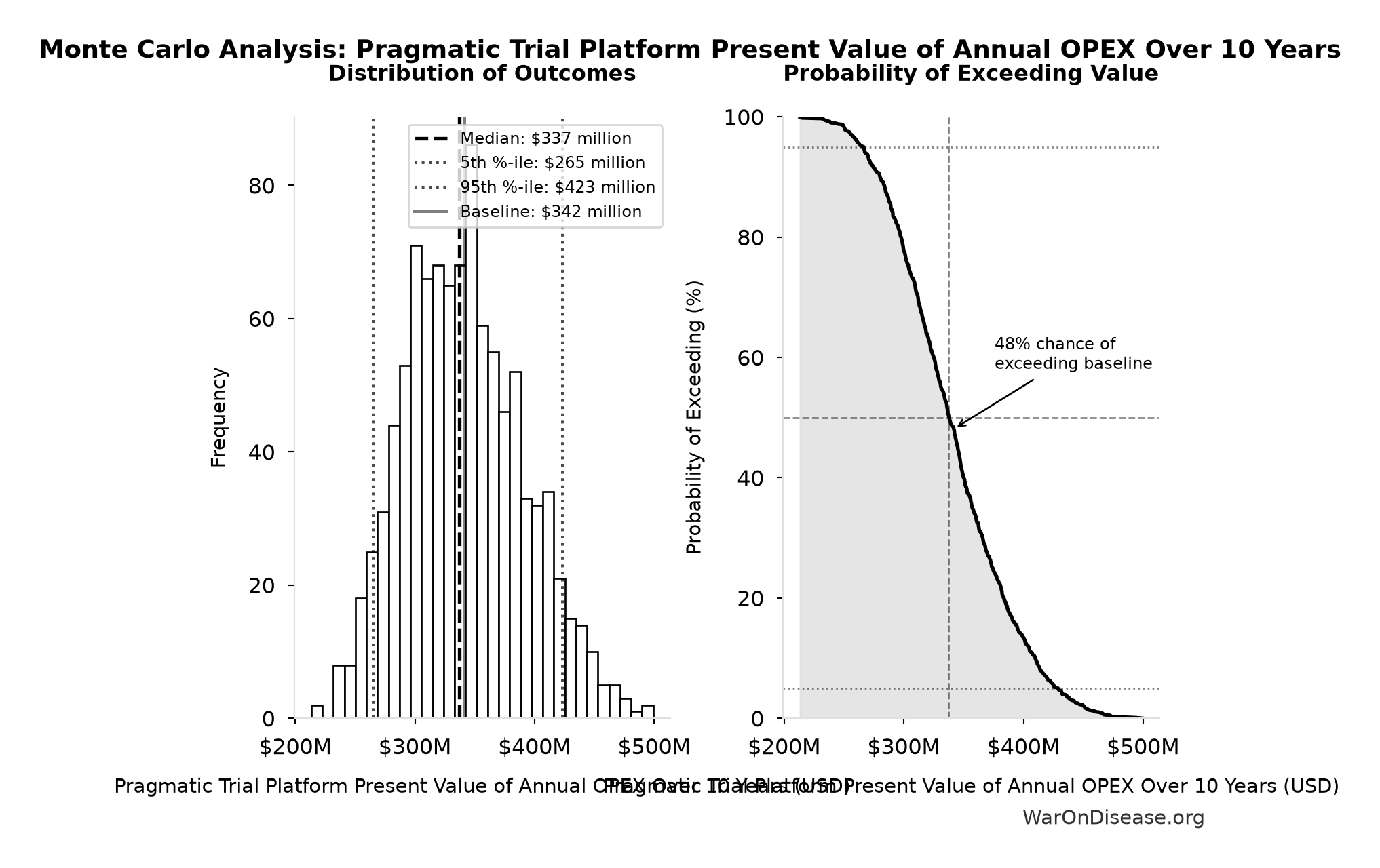
Simulation Results Summary: Pragmatic Trial Platform Present Value of Annual OPEX Over 10 Years
| Statistic | Value |
|---|---|
| Baseline (deterministic) | $342 million |
| Mean (expected value) | $340 million |
| Median (50th percentile) | $337 million |
| Standard Deviation | $48.2 million |
| 90% Range (5th-95th percentile) | [$265 million, $423 million] |
The histogram shows 1,000 of the 10,000 Monte Carlo draws for Pragmatic Trial Platform Present Value of Annual OPEX Over 10 Years; the summary statistics use all 10,000. The exceedance curve (right) shows the probability of the outcome exceeding any given value.
Exceedance Probability
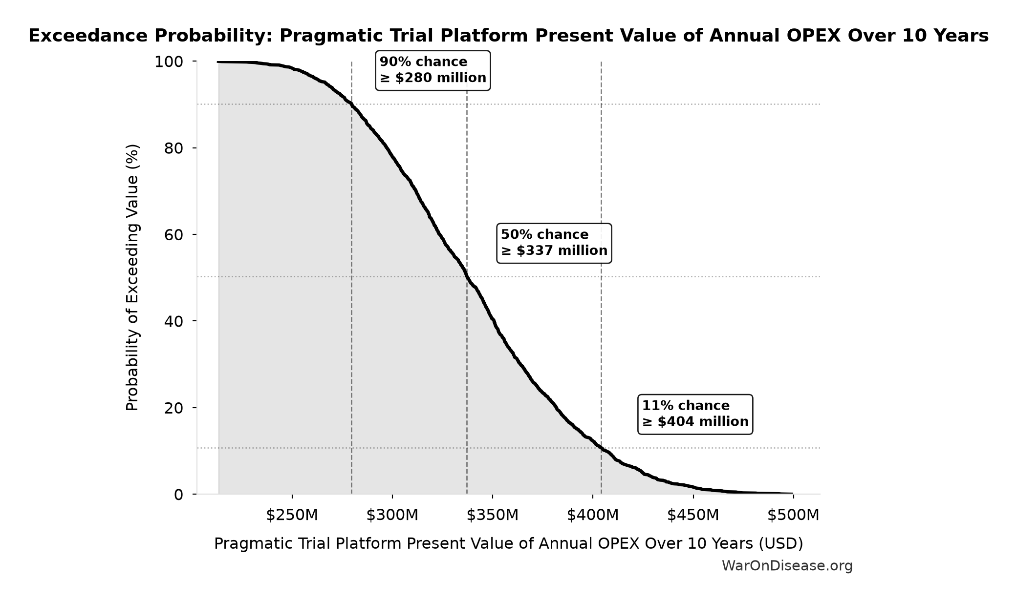
This exceedance probability chart shows the likelihood that Pragmatic Trial Platform Present Value of Annual OPEX Over 10 Years will exceed any given threshold. The higher the curve at a threshold, the more likely the value exceeds it.
Pragmatic Trial Platform Total NPV Cost: $611 million
Note📊 Details
Total NPV cost (upfront + PV of annual opex)
Inputs:
- Pragmatic Trial Platform Present Value of Annual OPEX Over 10 Years 🔢: $342 million
- Pragmatic Trial Platform Total NPV Upfront Costs 🔢: $270 million
\[ \begin{gathered} Cost_{platform,total} \\ = PV_{OPEX} + Cost_{upfront,total} \\ = \$342M + \$270M \\ = \$611M \end{gathered} \] where: \[ \begin{gathered} PV_{OPEX} \\ = \frac{T_{horizon}}{OPEX_{total} \times r_{discount}} \\ = \frac{10}{\$40M \times 3\%} \\ = \$342M \end{gathered} \] where: \[ \begin{gathered} OPEX_{total} \\ = OPEX_{ann} + OPEX_{DIH,ann} \\ = \$18.9M + \$21.1M \\ = \$40M \end{gathered} \] where: \[ \begin{gathered} Cost_{upfront,total} \\ = Cost_{upfront} + Cost_{DIH,init} \\ = \$40M + \$230M \\ = \$270M \end{gathered} \] ✓ High confidence
Sensitivity Analysis
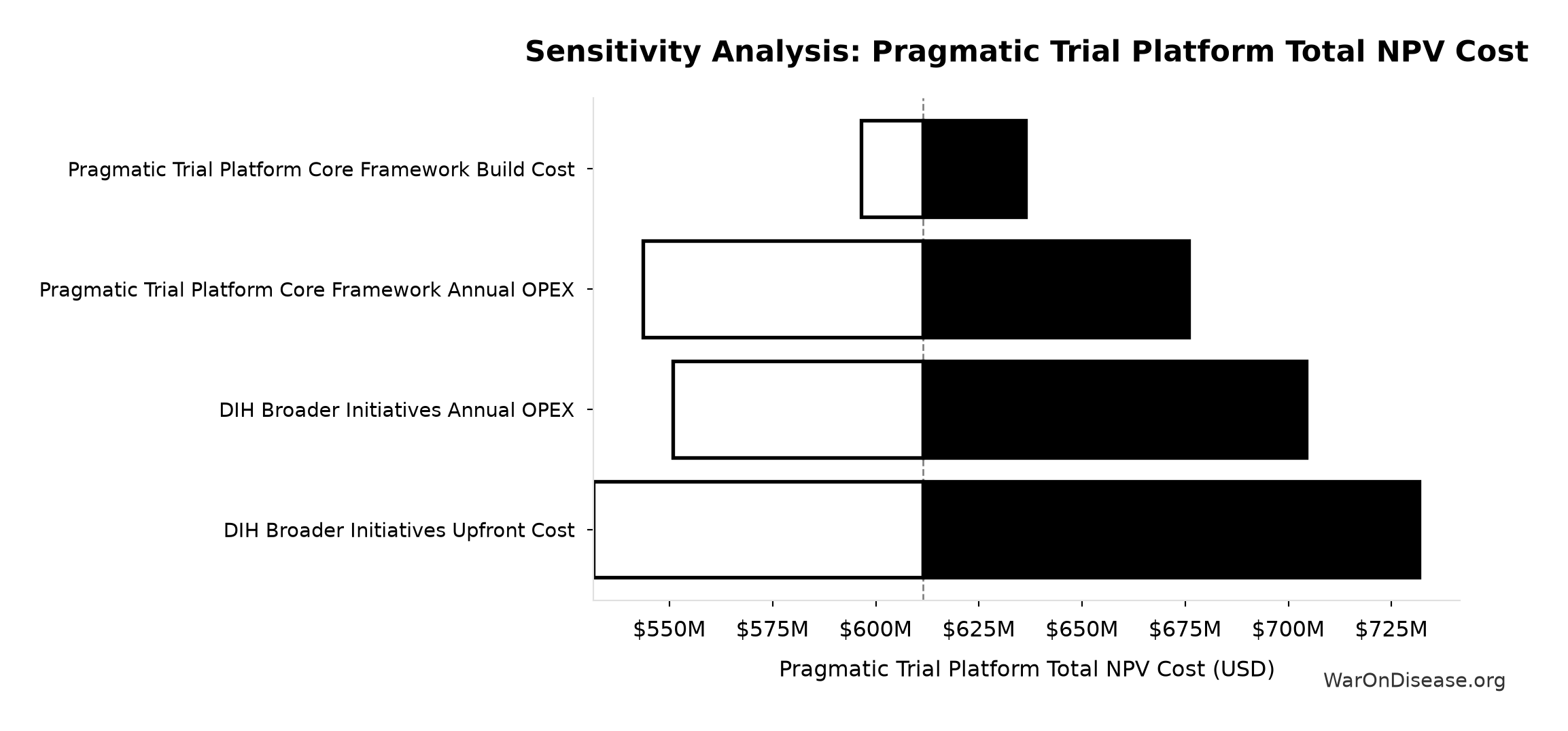
Sensitivity Indices for Pragmatic Trial Platform Total NPV Cost
Regression-based sensitivity showing which inputs explain the most variance in the output.
| Input Parameter | Sensitivity Coefficient | Interpretation |
|---|---|---|
| Pragmatic Trial Platform Total NPV Upfront Costs (USD) | 0.7087 | Strong driver |
| Pragmatic Trial Platform Present Value of Annual OPEX Over 10 Years (USD) | 0.6952 | Strong driver |
Interpretation: Standardized coefficients show the change in output (in SD units) per 1 SD change in input. Values near ±1 indicate strong influence; values exceeding ±1 may occur with correlated inputs.
Monte Carlo Distribution
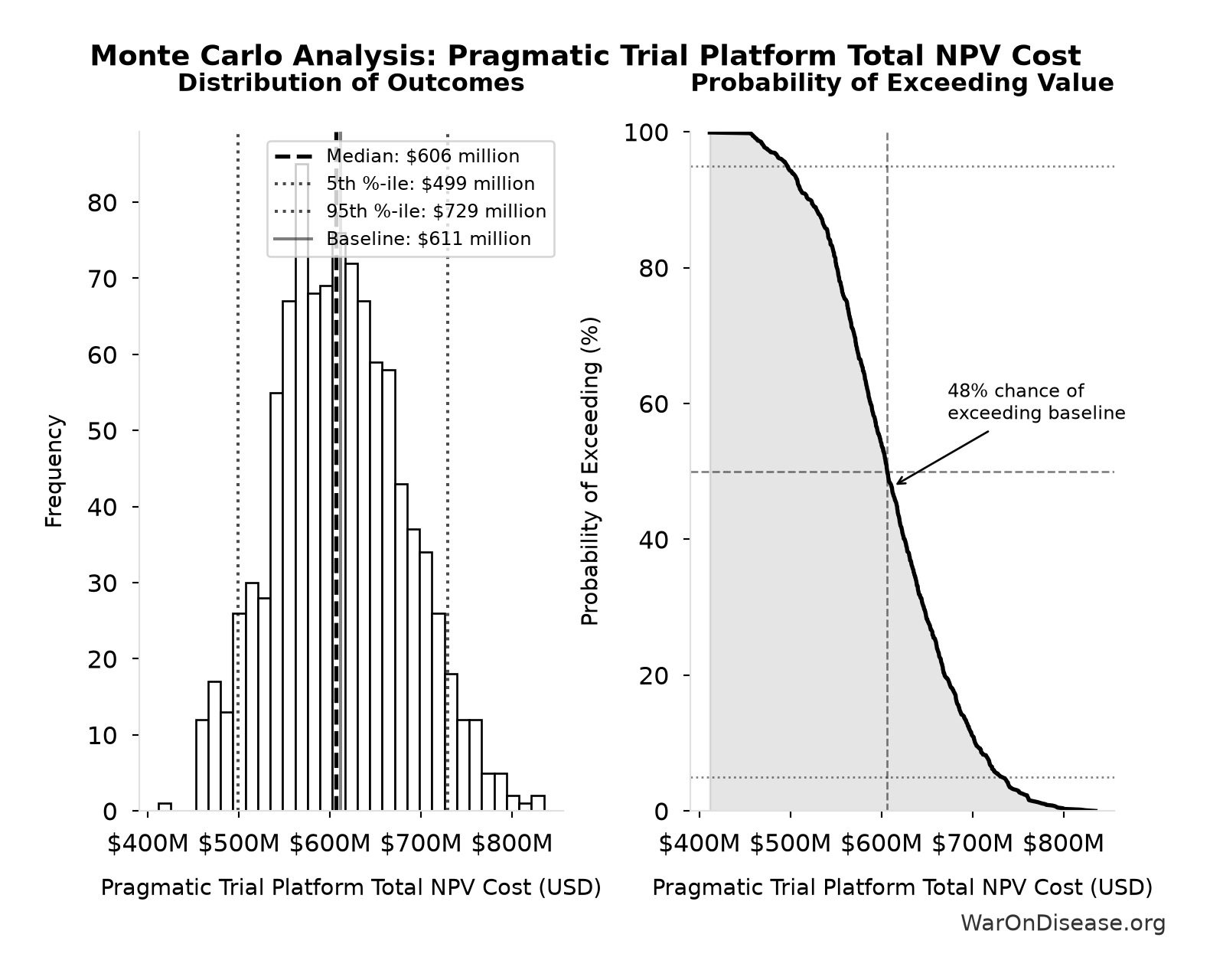
Simulation Results Summary: Pragmatic Trial Platform Total NPV Cost
| Statistic | Value |
|---|---|
| Baseline (deterministic) | $611 million |
| Mean (expected value) | $609 million |
| Median (50th percentile) | $606 million |
| Standard Deviation | $69.3 million |
| 90% Range (5th-95th percentile) | [$499 million, $729 million] |
The histogram shows 1,000 of the 10,000 Monte Carlo draws for Pragmatic Trial Platform Total NPV Cost; the summary statistics use all 10,000. The exceedance curve (right) shows the probability of the outcome exceeding any given value.
Exceedance Probability
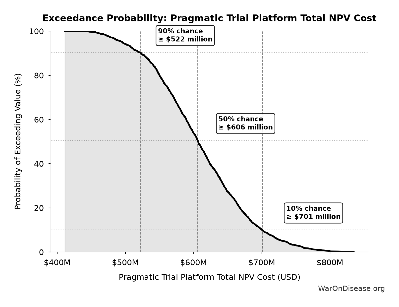
This exceedance probability chart shows the likelihood that Pragmatic Trial Platform Total NPV Cost will exceed any given threshold. The higher the curve at a threshold, the more likely the value exceeds it.
Pragmatic Trial Platform Total NPV Upfront Costs: $270 million
Note📊 Details
Total NPV upfront costs (pragmatic trial platform core + DIH initiatives)
Inputs:
- Pragmatic Trial Platform Core Framework Build Cost: $40 million (95% CI: $25 million - $65 million)
- DIH Broader Initiatives Upfront Cost: $230 million (95% CI: $150 million - $350 million)
\[ \begin{gathered} Cost_{upfront,total} \\ = Cost_{upfront} + Cost_{DIH,init} \\ = \$40M + \$230M \\ = \$270M \end{gathered} \]
✓ High confidence
Sensitivity Analysis
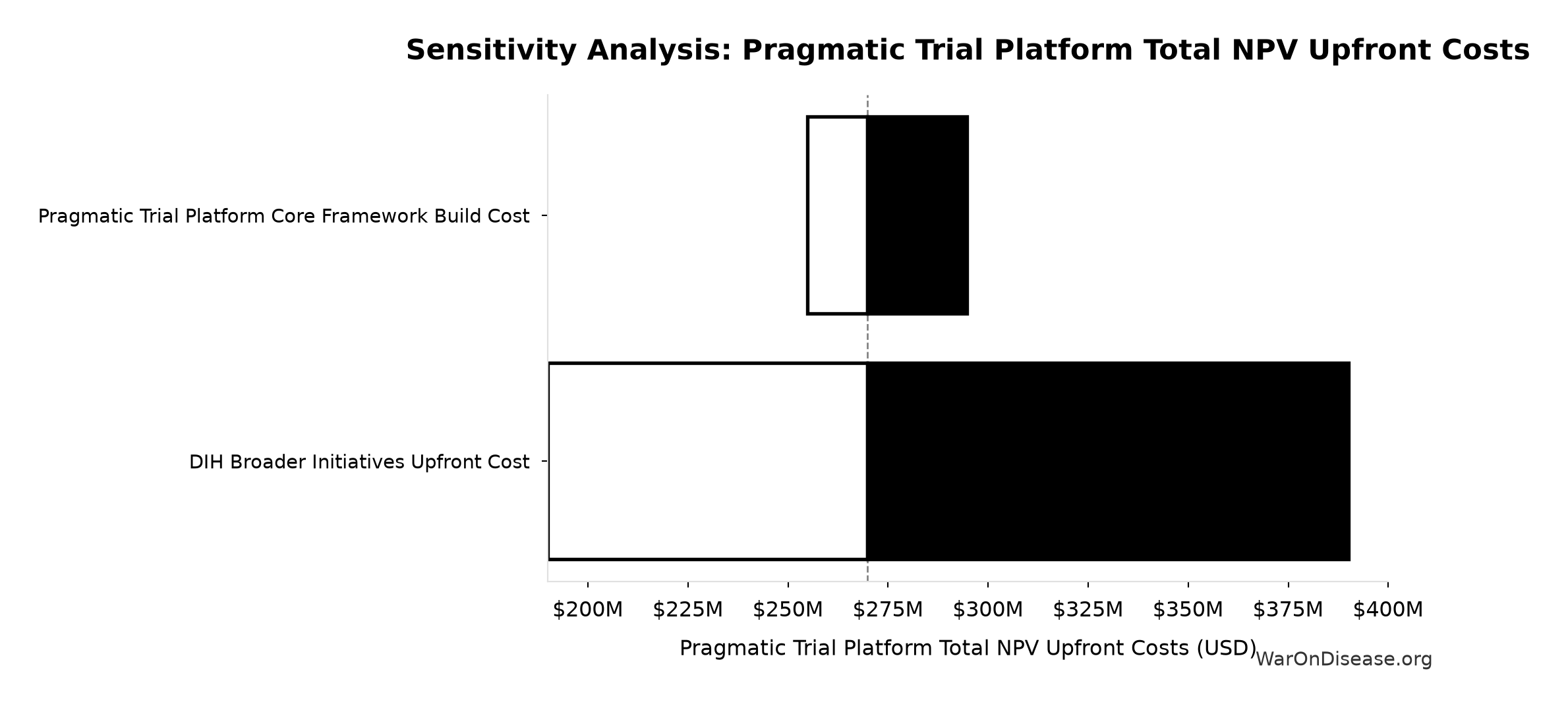
Sensitivity Indices for Pragmatic Trial Platform Total NPV Upfront Costs
Regression-based sensitivity showing which inputs explain the most variance in the output.
| Input Parameter | Sensitivity Coefficient | Interpretation |
|---|---|---|
| DIH Broader Initiatives Upfront Cost (USD) | 0.9826 | Strong driver |
| Pragmatic Trial Platform Core Framework Build Cost (USD) | 0.1958 | Weak driver |
Interpretation: Standardized coefficients show the change in output (in SD units) per 1 SD change in input. Values near ±1 indicate strong influence; values exceeding ±1 may occur with correlated inputs.
Monte Carlo Distribution
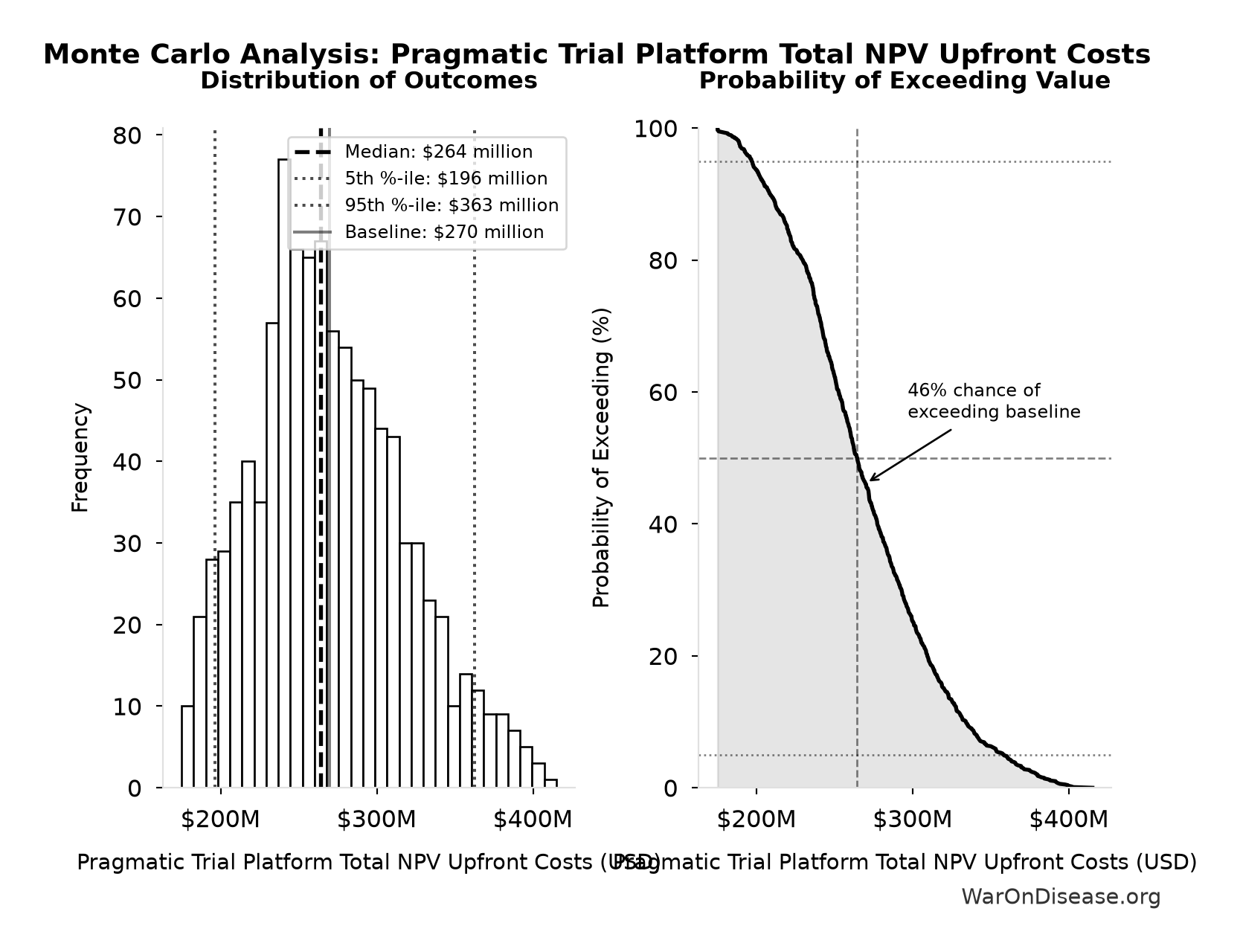
Simulation Results Summary: Pragmatic Trial Platform Total NPV Upfront Costs
| Statistic | Value |
|---|---|
| Baseline (deterministic) | $270 million |
| Mean (expected value) | $269 million |
| Median (50th percentile) | $264 million |
| Standard Deviation | $49.1 million |
| 90% Range (5th-95th percentile) | [$196 million, $363 million] |
The histogram shows 1,000 of the 10,000 Monte Carlo draws for Pragmatic Trial Platform Total NPV Upfront Costs; the summary statistics use all 10,000. The exceedance curve (right) shows the probability of the outcome exceeding any given value.
Exceedance Probability
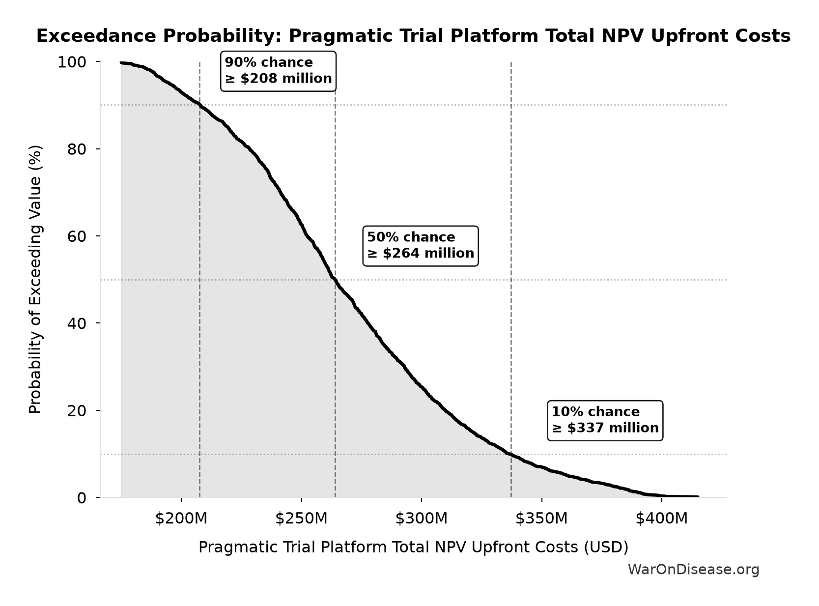
This exceedance probability chart shows the likelihood that Pragmatic Trial Platform Total NPV Upfront Costs will exceed any given threshold. The higher the curve at a threshold, the more likely the value exceeds it.
Patients Fundable Annually at Reference Funding: 23.4 million patients/year
Note📊 Details
Number of patients fundable annually at the reference pragmatic trial funding level and empirical pragmatic trial cost. Source-agnostic counterpart of DIH_PATIENTS_FUNDABLE_ANNUALLY.
Inputs:
- Reference Annual Trial Subsidies 🔢: $21.8 billion
- Pragmatic Trial Cost per Patient 📊: $929 (95% CI: $97 - $3,000)
\[ \begin{gathered} N_{fundable,ref} \\ = \frac{Subsidies_{trial,ref}}{Cost_{pragmatic,pt}} \\ = \frac{\$21.8B}{\$929} \\ = 23.4M \end{gathered} \] where: \[ \begin{gathered} Subsidies_{trial,ref} \\ = Funding_{trial,ref} - OPEX_{trial} \\ = \$21.8B - \$40M \\ = \$21.8B \end{gathered} \] where: \[ \begin{gathered} OPEX_{trial} \\ = Cost_{platform} + Cost_{staff} + Cost_{infra} \\ + Cost_{regulatory} + Cost_{community} \\ = \$15M + \$10M + \$8M + \$5M + \$2M \\ = \$40M \end{gathered} \] ✓ High confidence
Sensitivity Analysis
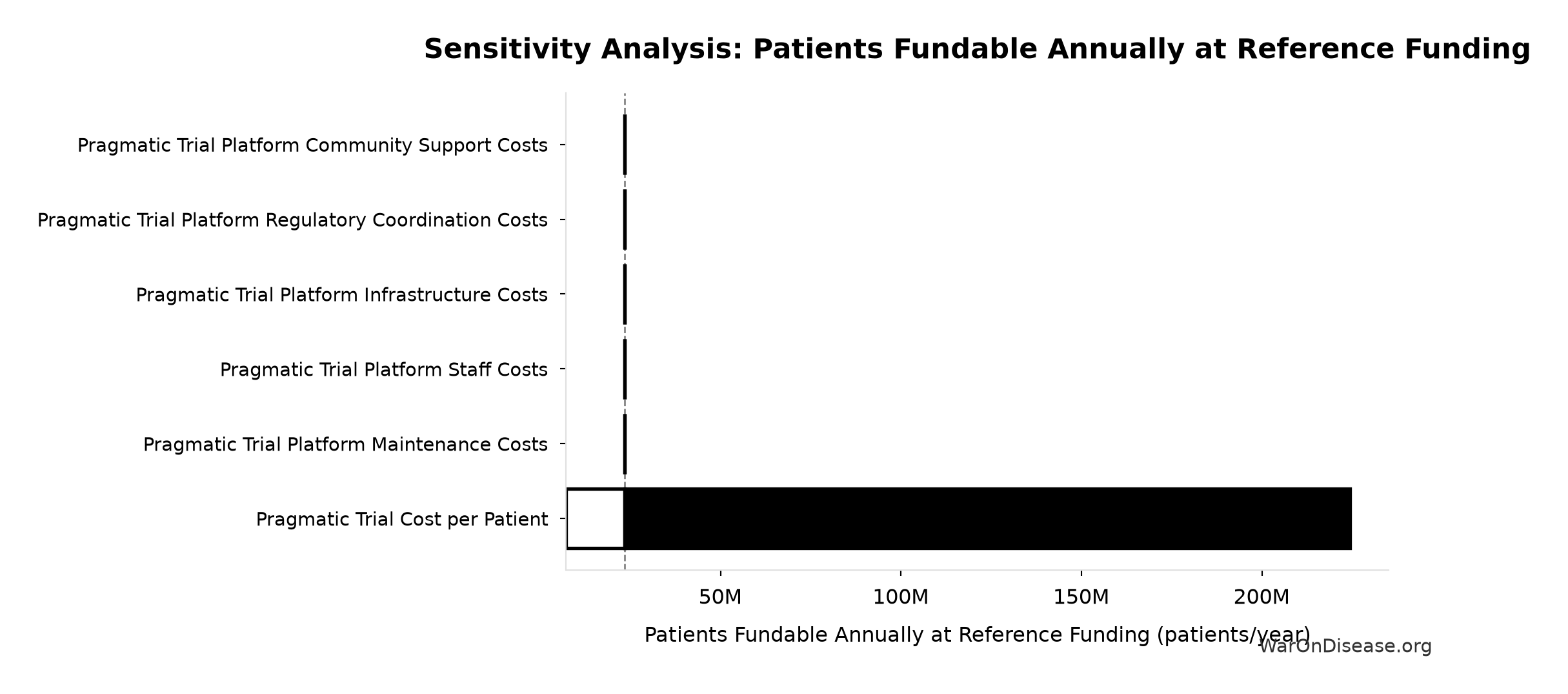
Sensitivity Indices for Patients Fundable Annually at Reference Funding
Regression-based sensitivity showing which inputs explain the most variance in the output.
| Input Parameter | Sensitivity Coefficient | Interpretation |
|---|---|---|
| Pragmatic Trial Cost per Patient (USD/patient) | -0.6862 | Strong driver |
| Reference Annual Trial Subsidies (USD/year) | 0.0014 | Minimal effect |
Interpretation: Standardized coefficients show the change in output (in SD units) per 1 SD change in input. Values near ±1 indicate strong influence; values exceeding ±1 may occur with correlated inputs.
Monte Carlo Distribution
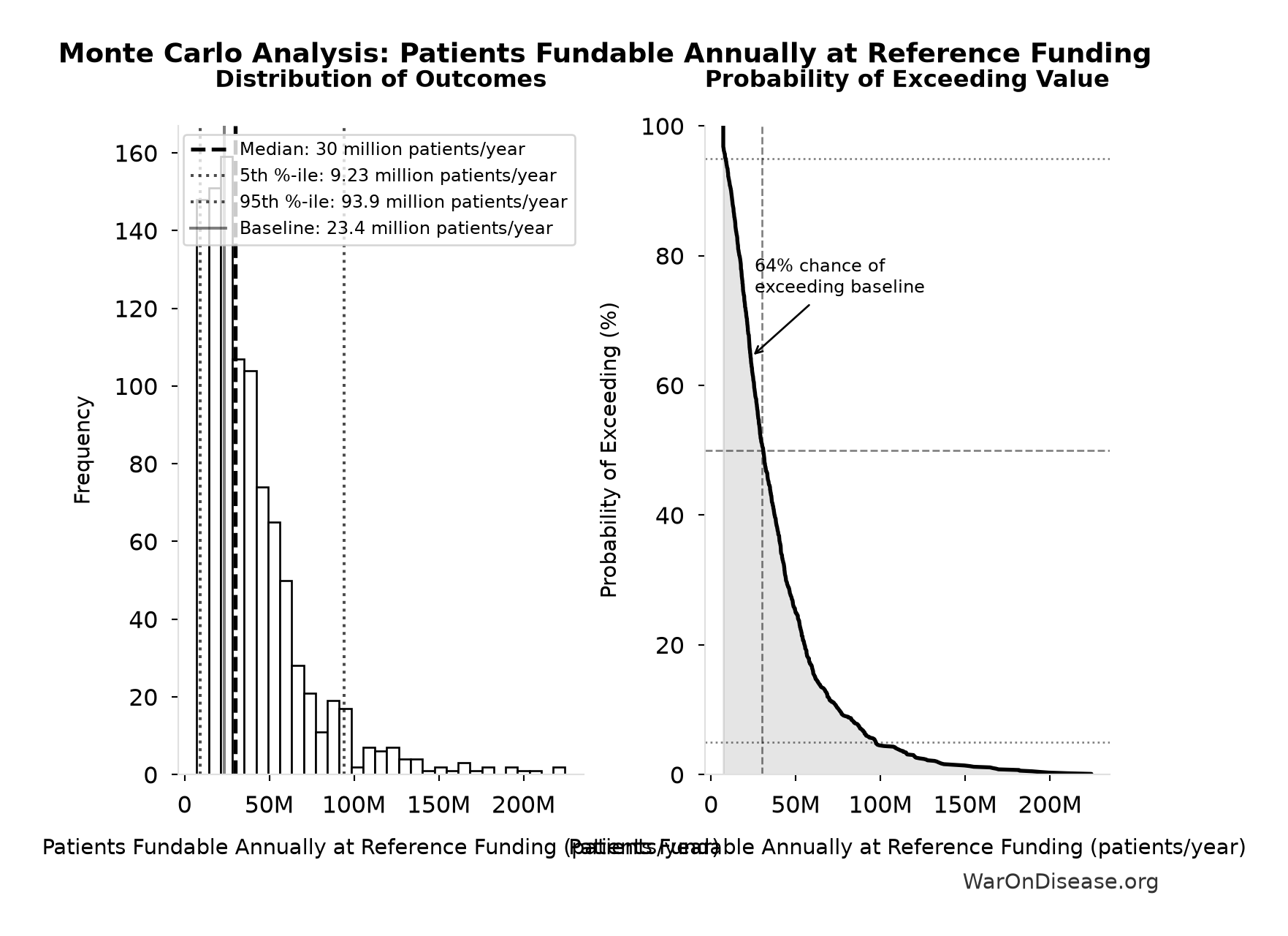
Simulation Results Summary: Patients Fundable Annually at Reference Funding
| Statistic | Value |
|---|---|
| Baseline (deterministic) | 23.4 million |
| Mean (expected value) | 38.4 million |
| Median (50th percentile) | 30 million |
| Standard Deviation | 29.5 million |
| 90% Range (5th-95th percentile) | [9.23 million, 93.9 million] |
The histogram shows 1,000 of the 10,000 Monte Carlo draws for Patients Fundable Annually at Reference Funding; the summary statistics use all 10,000. The exceedance curve (right) shows the probability of the outcome exceeding any given value.
Exceedance Probability
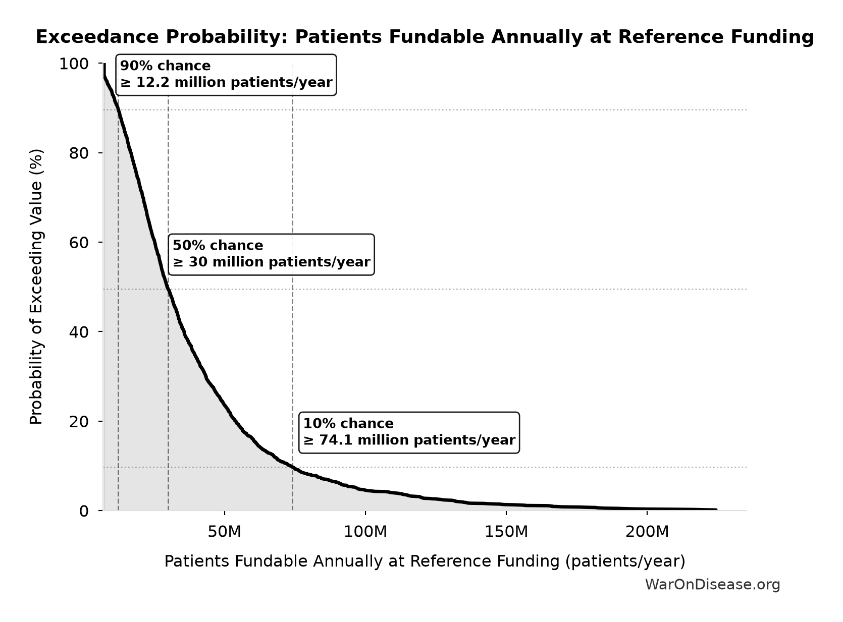
This exceedance probability chart shows the likelihood that Patients Fundable Annually at Reference Funding will exceed any given threshold. The higher the curve at a threshold, the more likely the value exceeds it.
Therapeutic Space Exploration Time at Treaty-Scale Trial Capacity: 36 years
Note📊 Details
Years to explore the entire therapeutic search space with treaty-scale pragmatic trial capacity. At increased discovery rate, finding first treatments for all currently untreatable diseases takes ~36 years instead of ~443.
Inputs:
- Status Quo Therapeutic Space Exploration Time 🔢: 443 years
- Pragmatic Trial Capacity Multiplier at Treaty-Scale Funding 🔢: 12.3x
\[ \begin{gathered} T_{queue,trial} \\ = \frac{T_{queue,SQ}}{k_{capacity}} \\ = \frac{443}{12.3} \\ = 36 \end{gathered} \] where: \[ \begin{gathered} T_{queue,SQ} \\ = \frac{N_{untreated}}{Treatments_{new,ann}} \\ = \frac{6{,}650}{15} \\ = 443 \end{gathered} \] where: \[ \begin{gathered} N_{untreated} \\ = N_{rare} \times 0.95 \\ = 7{,}000 \times 0.95 \\ = 6{,}650 \end{gathered} \] where: \[ \begin{gathered} k_{capacity} \\ = \frac{N_{fundable,ref}}{Slots_{curr}} \\ = \frac{23.4M}{1.9M} \\ = 12.3 \end{gathered} \] where: \[ \begin{gathered} N_{fundable,ref} \\ = \frac{Subsidies_{trial,ref}}{Cost_{pragmatic,pt}} \\ = \frac{\$21.8B}{\$929} \\ = 23.4M \end{gathered} \] where: \[ \begin{gathered} Subsidies_{trial,ref} \\ = Funding_{trial,ref} - OPEX_{trial} \\ = \$21.8B - \$40M \\ = \$21.8B \end{gathered} \] where: \[ \begin{gathered} OPEX_{trial} \\ = Cost_{platform} + Cost_{staff} + Cost_{infra} \\ + Cost_{regulatory} + Cost_{community} \\ = \$15M + \$10M + \$8M + \$5M + \$2M \\ = \$40M \end{gathered} \] ? Low confidence
Sensitivity Analysis
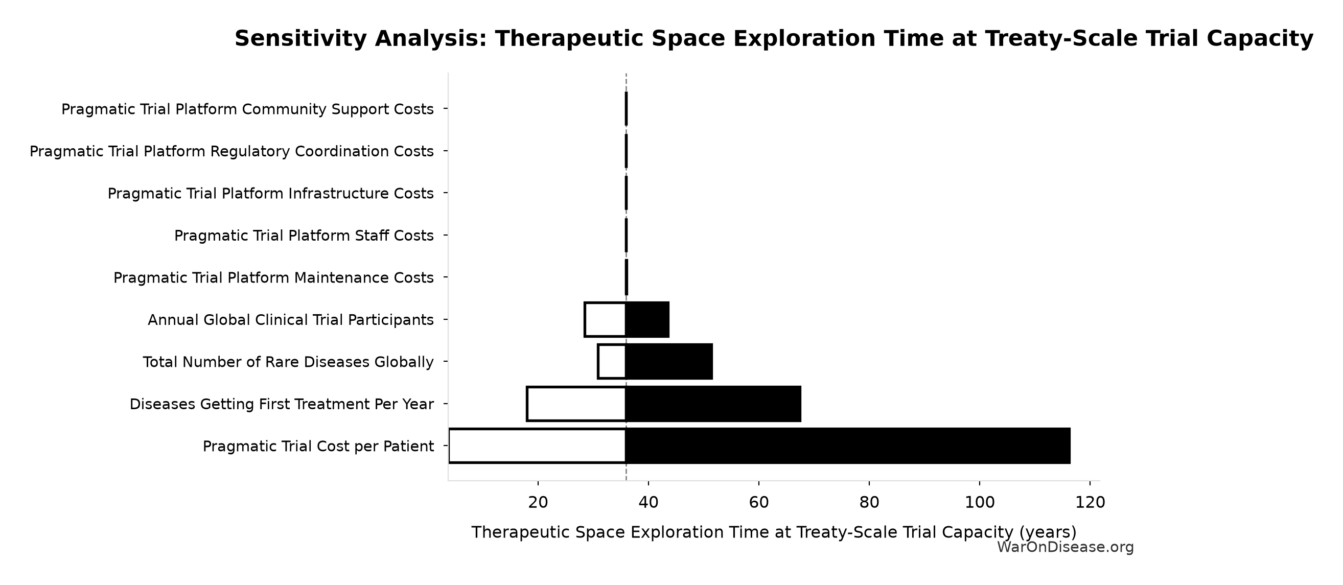
Sensitivity Indices for Therapeutic Space Exploration Time at Treaty-Scale Trial Capacity
Regression-based sensitivity showing which inputs explain the most variance in the output.
| Input Parameter | Sensitivity Coefficient | Interpretation |
|---|---|---|
| Pragmatic Trial Capacity Multiplier at Treaty-Scale Funding (x) | -0.5900 | Strong driver |
| Status Quo Therapeutic Space Exploration Time (years) | 0.4217 | Moderate driver |
Interpretation: Standardized coefficients show the change in output (in SD units) per 1 SD change in input. Values near ±1 indicate strong influence; values exceeding ±1 may occur with correlated inputs.
Monte Carlo Distribution
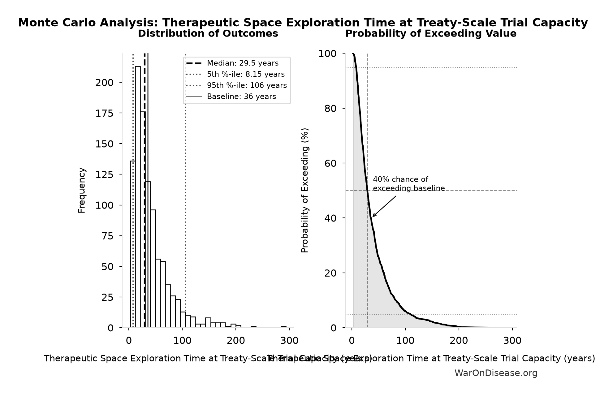
Simulation Results Summary: Therapeutic Space Exploration Time at Treaty-Scale Trial Capacity
| Statistic | Value |
|---|---|
| Baseline (deterministic) | 36 |
| Mean (expected value) | 39.5 |
| Median (50th percentile) | 29.5 |
| Standard Deviation | 32.9 |
| 90% Range (5th-95th percentile) | [8.15, 106] |
The histogram shows 1,000 of the 10,000 Monte Carlo draws for Therapeutic Space Exploration Time at Treaty-Scale Trial Capacity; the summary statistics use all 10,000. The exceedance curve (right) shows the probability of the outcome exceeding any given value.
Exceedance Probability
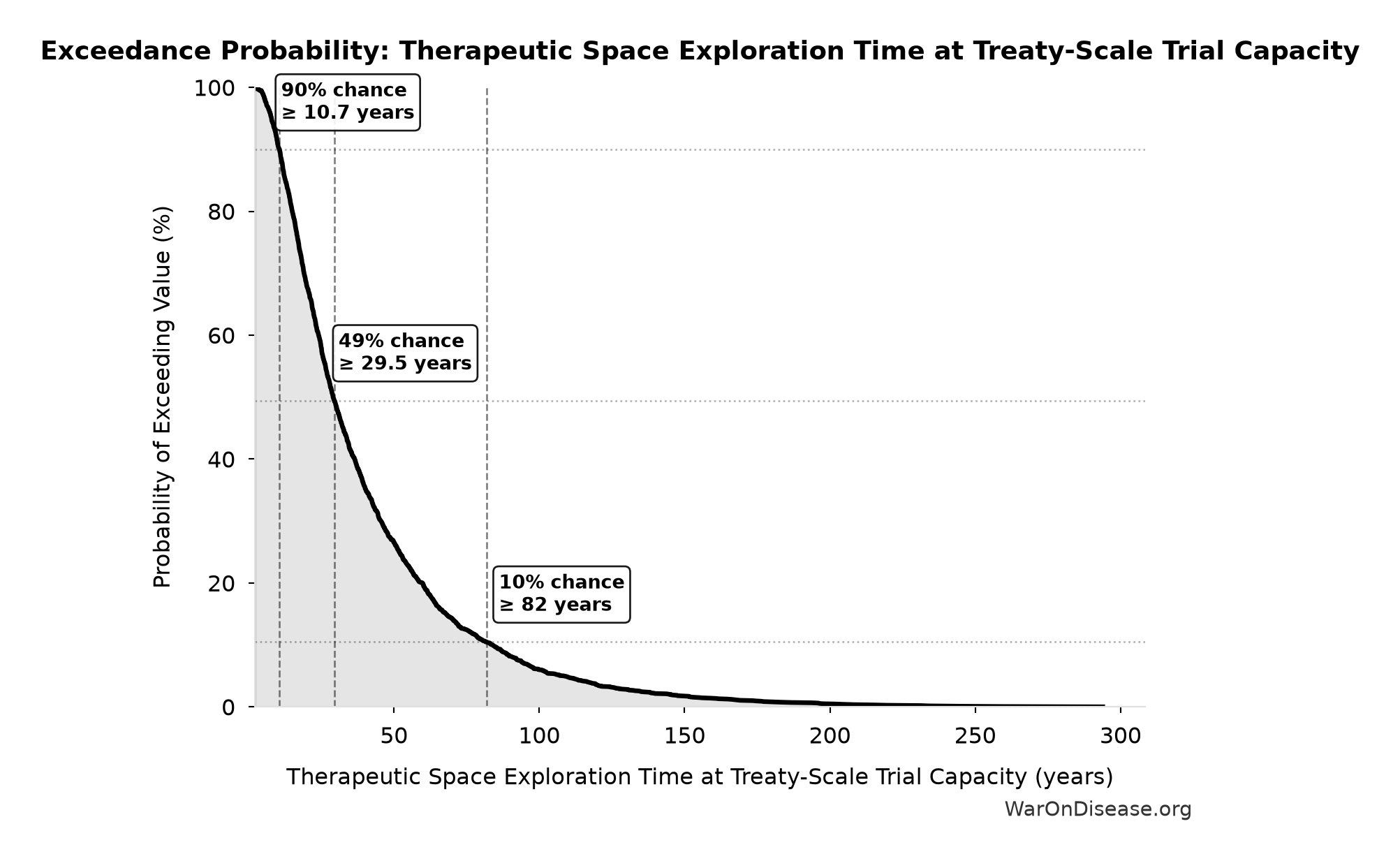
This exceedance probability chart shows the likelihood that Therapeutic Space Exploration Time at Treaty-Scale Trial Capacity will exceed any given threshold. The higher the curve at a threshold, the more likely the value exceeds it.
ROI from Pragmatic Trial R&D Savings Only: 439:1
Note📊 Details
ROI from pragmatic trial R&D savings only (10-year NPV, most conservative estimate)
Inputs:
- NPV of Pragmatic Trial Benefits (R&D Only, 10-Year Discounted) 🔢: $269 billion
- Pragmatic Trial Platform Total NPV Cost 🔢: $611 million
\[ \begin{gathered} ROI_{RD} \\ = \frac{NPV_{RD}}{Cost_{platform,total}} \\ = \frac{\$269B}{\$611M} \\ = 439 \end{gathered} \] where: \[ \begin{gathered} NPV_{RD} \\ = \sum_{t=1}^{10} \frac{Savings_{RD,ann} \cdot \frac{\min(t,5)}{5}}{(1+r)^t} \end{gathered} \] where: \[ \begin{gathered} Savings_{RD,ann} \\ = Benefit_{RD,ann} - OPEX_{trial} \\ = \$40.5B - \$40M \\ = \$40.4B \end{gathered} \] where: \[ \begin{gathered} Benefit_{RD,ann} \\ = Spending_{trials} \times Pct_{P2+P3} \times Reduce_{pct} \\ = \$60B \times 69\% \times 97.7\% \\ = \$40.5B \end{gathered} \] where: \[ \begin{gathered} Reduce_{pct} \\ = 1 - \frac{Cost_{pragmatic,pt}}{Cost_{P3,pt}} \\ = 1 - \frac{\$929}{\$41K} \\ = 97.7\% \end{gathered} \] where: \[ \begin{gathered} OPEX_{trial} \\ = Cost_{platform} + Cost_{staff} + Cost_{infra} \\ + Cost_{regulatory} + Cost_{community} \\ = \$15M + \$10M + \$8M + \$5M + \$2M \\ = \$40M \end{gathered} \] where: \[ \begin{gathered} Cost_{platform,total} \\ = PV_{OPEX} + Cost_{upfront,total} \\ = \$342M + \$270M \\ = \$611M \end{gathered} \] where: \[ \begin{gathered} PV_{OPEX} \\ = \frac{T_{horizon}}{OPEX_{total} \times r_{discount}} \\ = \frac{10}{\$40M \times 3\%} \\ = \$342M \end{gathered} \] where: \[ \begin{gathered} OPEX_{total} \\ = OPEX_{ann} + OPEX_{DIH,ann} \\ = \$18.9M + \$21.1M \\ = \$40M \end{gathered} \] where: \[ \begin{gathered} Cost_{upfront,total} \\ = Cost_{upfront} + Cost_{DIH,init} \\ = \$40M + \$230M \\ = \$270M \end{gathered} \] ✓ High confidence
Sensitivity Analysis
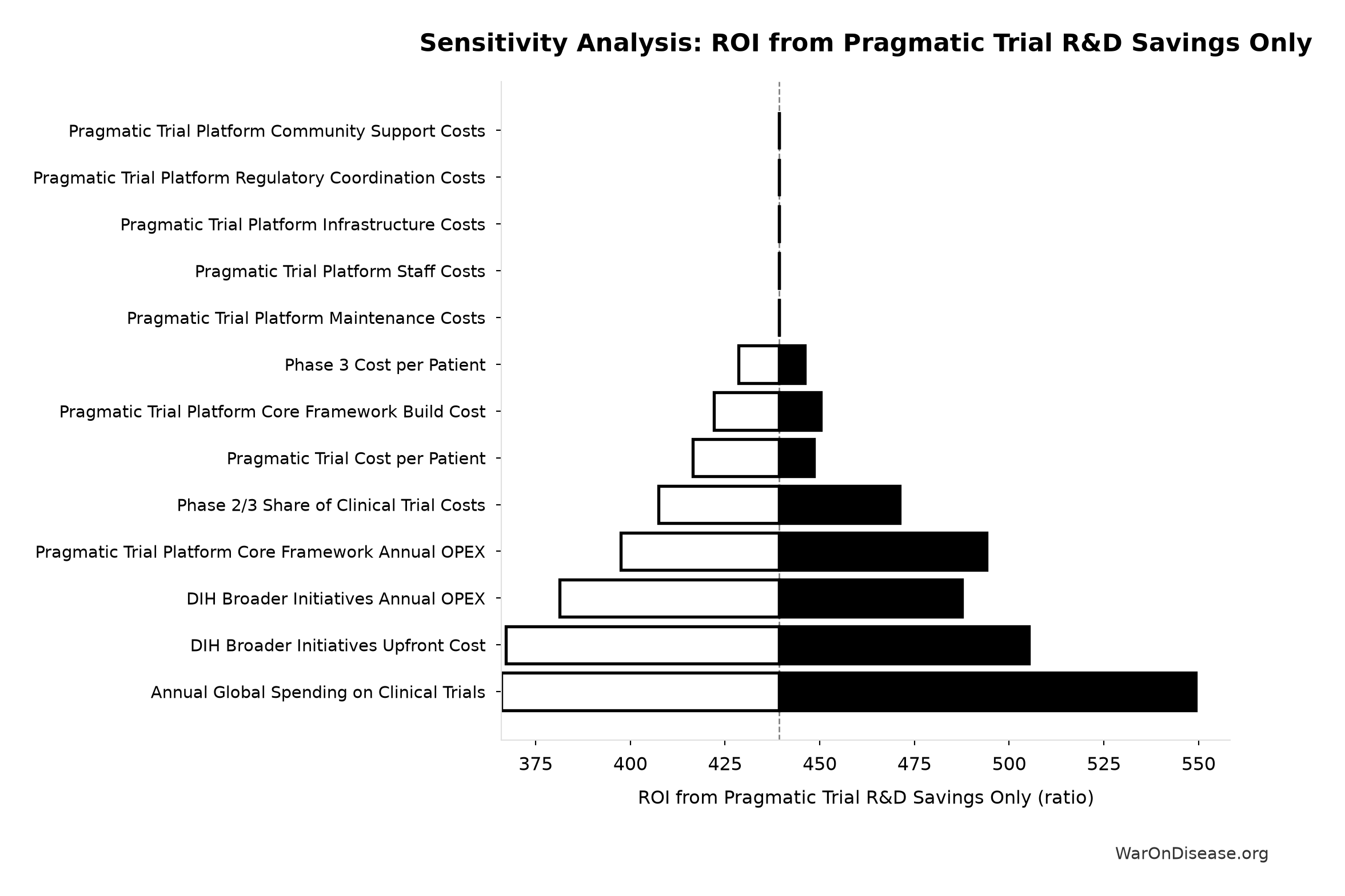
Sensitivity Indices for ROI from Pragmatic Trial R&D Savings Only
Regression-based sensitivity showing which inputs explain the most variance in the output.
| Input Parameter | Sensitivity Coefficient | Interpretation |
|---|---|---|
| NPV of Pragmatic Trial Benefits (R&D Only, 10-Year Discounted) (USD) | 0.8007 | Strong driver |
| Pragmatic Trial Platform Total NPV Cost (USD) | -0.5884 | Strong driver |
Interpretation: Standardized coefficients show the change in output (in SD units) per 1 SD change in input. Values near ±1 indicate strong influence; values exceeding ±1 may occur with correlated inputs.
Monte Carlo Distribution
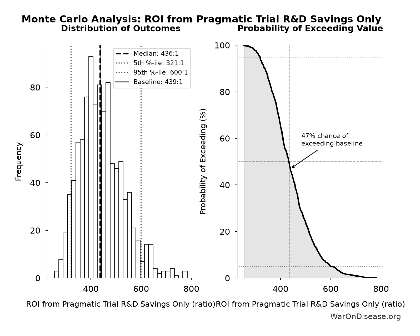
Simulation Results Summary: ROI from Pragmatic Trial R&D Savings Only
| Statistic | Value |
|---|---|
| Baseline (deterministic) | 439:1 |
| Mean (expected value) | 445:1 |
| Median (50th percentile) | 436:1 |
| Standard Deviation | 85.7:1 |
| 90% Range (5th-95th percentile) | [321:1, 600:1] |
The histogram shows 1,000 of the 10,000 Monte Carlo draws for ROI from Pragmatic Trial R&D Savings Only; the summary statistics use all 10,000. The exceedance curve (right) shows the probability of the outcome exceeding any given value.
Exceedance Probability
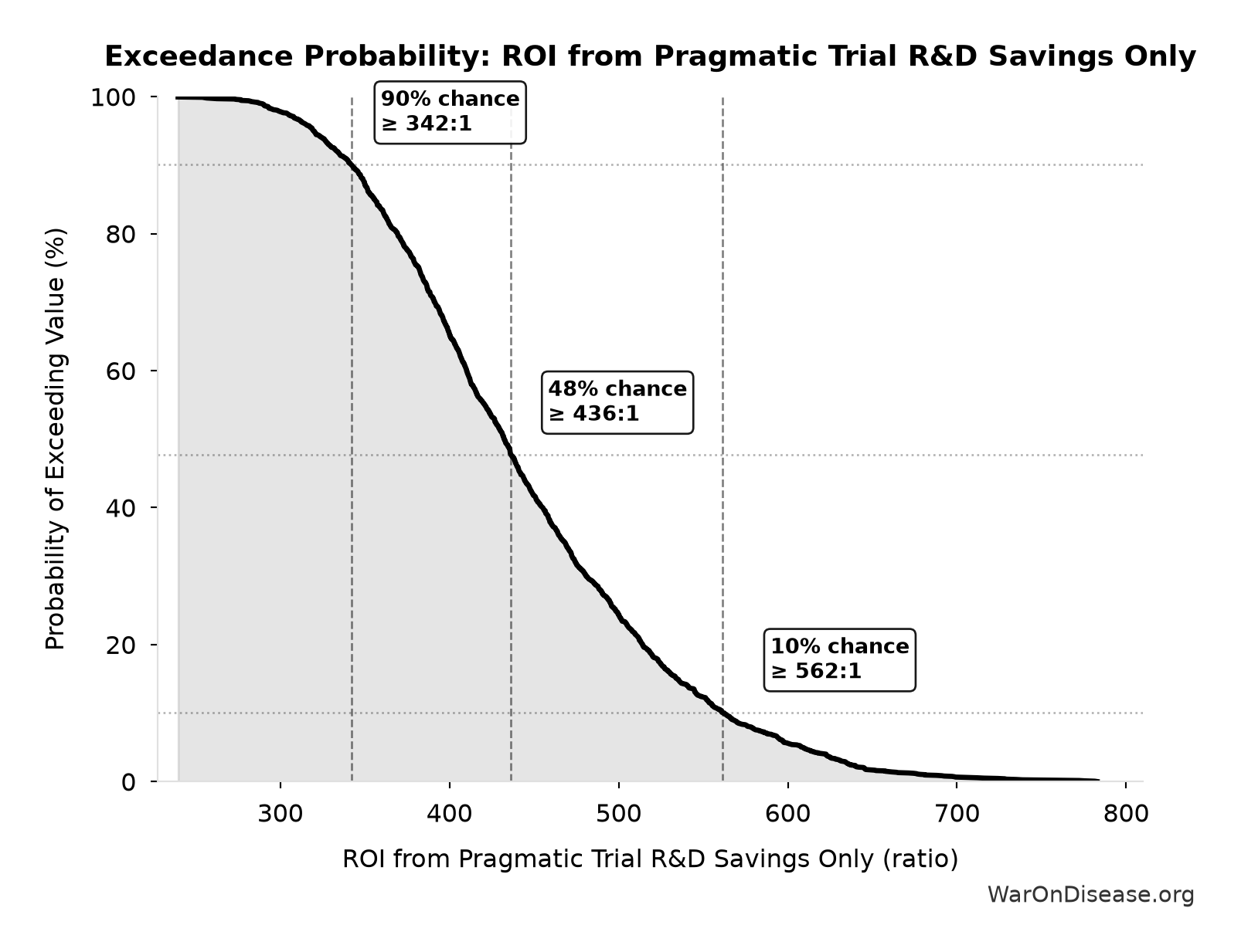
This exceedance probability chart shows the likelihood that ROI from Pragmatic Trial R&D Savings Only will exceed any given threshold. The higher the curve at a threshold, the more likely the value exceeds it.
Pragmatic Trial Capacity Multiplier at Treaty-Scale Funding: 12.3x
Note📊 Details
Trial capacity multiplier from treaty-scale pragmatic trial funding capacity vs. current global trial participation
Inputs:
- Annual Global Clinical Trial Participants 📊: 1.9 million patients/year (95% CI: 1.5 million patients/year - 2.3 million patients/year)
- Patients Fundable Annually at Reference Funding 🔢: 23.4 million patients/year
\[ \begin{gathered} k_{capacity} \\ = \frac{N_{fundable,ref}}{Slots_{curr}} \\ = \frac{23.4M}{1.9M} \\ = 12.3 \end{gathered} \] where: \[ \begin{gathered} N_{fundable,ref} \\ = \frac{Subsidies_{trial,ref}}{Cost_{pragmatic,pt}} \\ = \frac{\$21.8B}{\$929} \\ = 23.4M \end{gathered} \] where: \[ \begin{gathered} Subsidies_{trial,ref} \\ = Funding_{trial,ref} - OPEX_{trial} \\ = \$21.8B - \$40M \\ = \$21.8B \end{gathered} \] where: \[ \begin{gathered} OPEX_{trial} \\ = Cost_{platform} + Cost_{staff} + Cost_{infra} \\ + Cost_{regulatory} + Cost_{community} \\ = \$15M + \$10M + \$8M + \$5M + \$2M \\ = \$40M \end{gathered} \] ✓ High confidence
Sensitivity Analysis
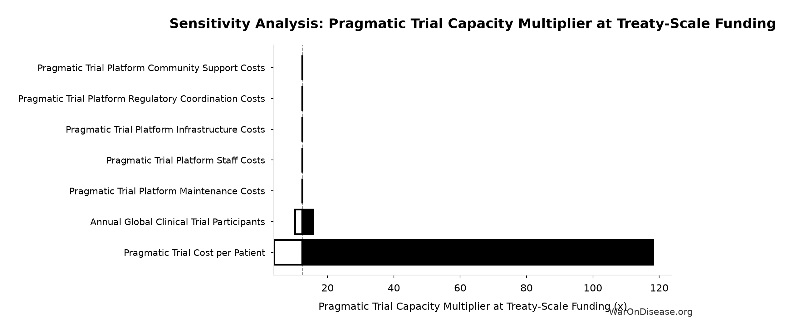
Sensitivity Indices for Pragmatic Trial Capacity Multiplier at Treaty-Scale Funding
Regression-based sensitivity showing which inputs explain the most variance in the output.
| Input Parameter | Sensitivity Coefficient | Interpretation |
|---|---|---|
| Patients Fundable Annually at Reference Funding (patients/year) | 0.9866 | Strong driver |
| Annual Global Clinical Trial Participants (patients/year) | -0.1314 | Weak driver |
Interpretation: Standardized coefficients show the change in output (in SD units) per 1 SD change in input. Values near ±1 indicate strong influence; values exceeding ±1 may occur with correlated inputs.
Monte Carlo Distribution
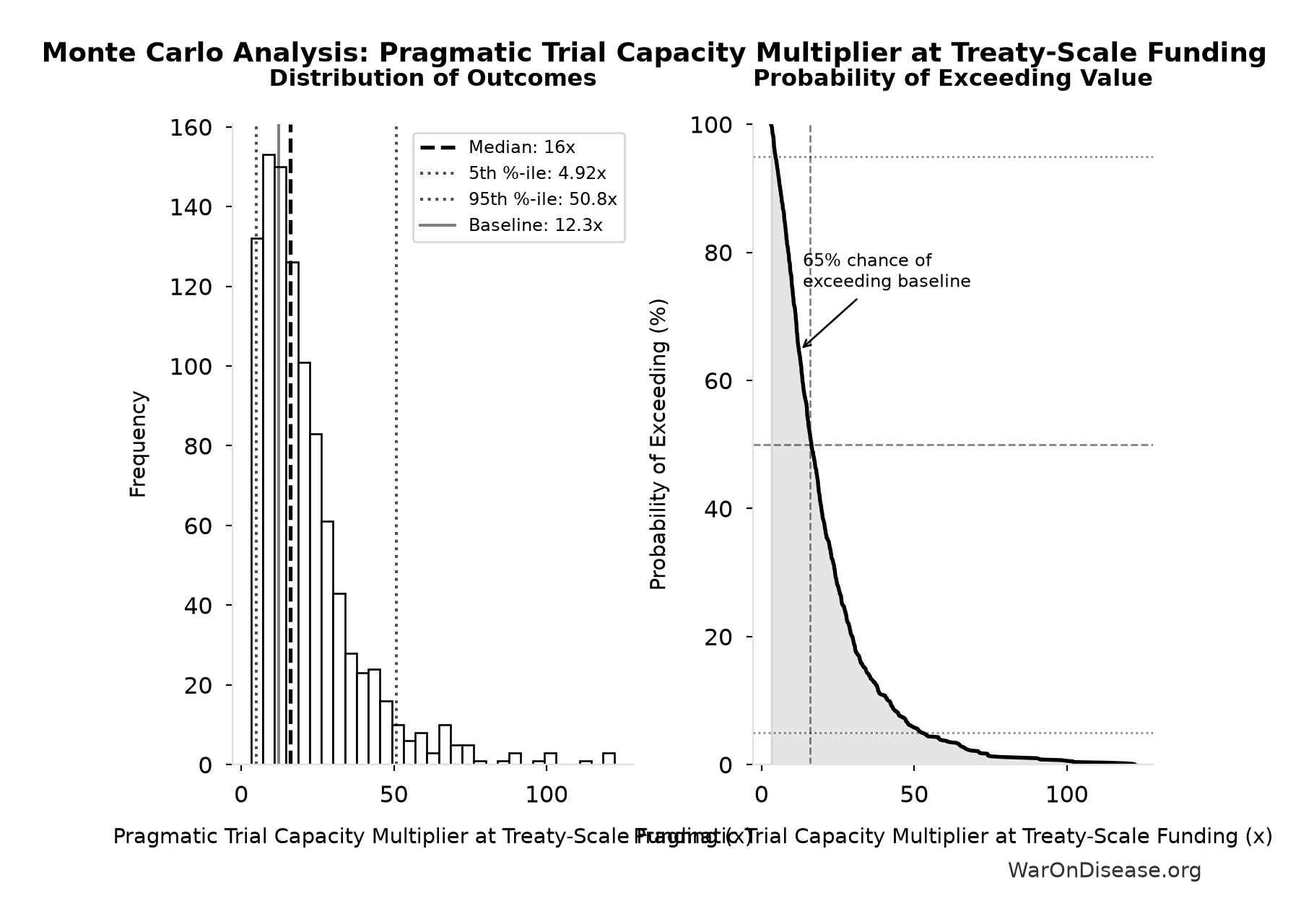
Simulation Results Summary: Pragmatic Trial Capacity Multiplier at Treaty-Scale Funding
| Statistic | Value |
|---|---|
| Baseline (deterministic) | 12.3x |
| Mean (expected value) | 20.5x |
| Median (50th percentile) | 16x |
| Standard Deviation | 16x |
| 90% Range (5th-95th percentile) | [4.92x, 50.8x] |
The histogram shows 1,000 of the 10,000 Monte Carlo draws for Pragmatic Trial Capacity Multiplier at Treaty-Scale Funding; the summary statistics use all 10,000. The exceedance curve (right) shows the probability of the outcome exceeding any given value.
Exceedance Probability
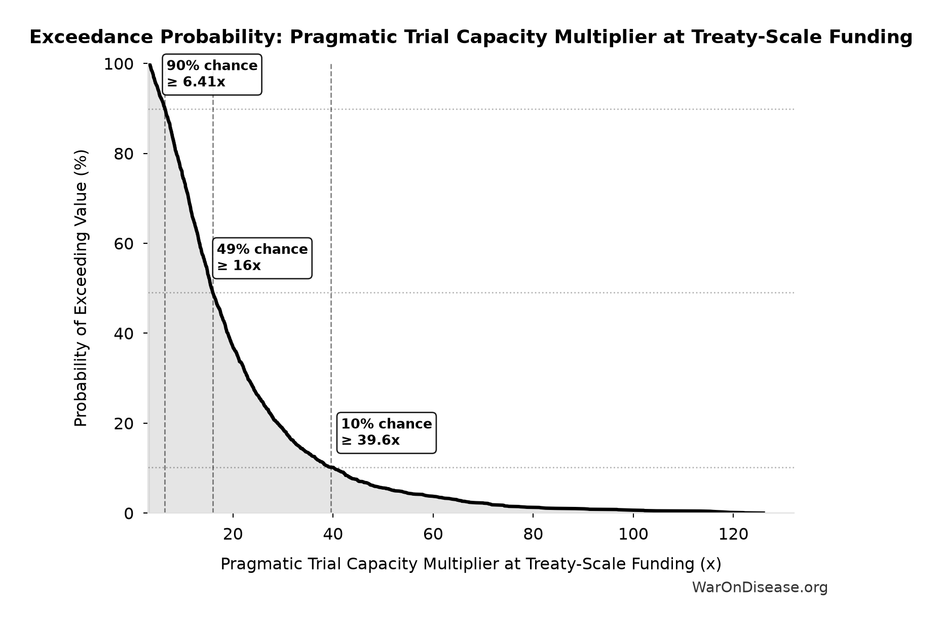
This exceedance probability chart shows the likelihood that Pragmatic Trial Capacity Multiplier at Treaty-Scale Funding will exceed any given threshold. The higher the curve at a threshold, the more likely the value exceeds it.
Total DALYs from Elimination of Efficacy Lag Plus Earlier Treatment Discovery from Higher Trial Throughput: 565 billion DALYs
Note📊 Details
Total DALYs averted from the combined treatment timeline shift. Calculated as annual global DALY burden × eventually avoidable percentage × timeline shift years. Includes both fatal and non-fatal diseases (WHO GBD methodology).
Inputs:
- Global Annual DALY Burden 📊: 2.88 billion DALYs/year (SE: ±150 million DALYs/year)
- Eventually Avoidable DALY Percentage: 92.6% (95% CI: 50% - 98%)
- Average Total Treatment Timeline Shift 🔢: 212 years
\[ \begin{gathered} DALYs_{max} \\ = DALYs_{global,ann} \times Pct_{avoid,DALY} \times T_{accel,max} \\ = 2.88B \times 92.6\% \times 212 \\ = 565B \end{gathered} \] where: \[ T_{accel,max} = T_{accel} + T_{lag} = 204 + 8.2 = 212 \] where: \[ \begin{gathered} T_{accel} \\ = T_{first,SQ} \times \left(1 - \frac{1}{k_{capacity}}\right) \\ = 222 \times \left(1 - \frac{1}{12.3}\right) \\ = 204 \end{gathered} \] where: \[ \begin{gathered} T_{first,SQ} \\ = T_{queue,SQ} \times 0.5 \\ = 443 \times 0.5 \\ = 222 \end{gathered} \] where: \[ \begin{gathered} T_{queue,SQ} \\ = \frac{N_{untreated}}{Treatments_{new,ann}} \\ = \frac{6{,}650}{15} \\ = 443 \end{gathered} \] where: \[ \begin{gathered} N_{untreated} \\ = N_{rare} \times 0.95 \\ = 7{,}000 \times 0.95 \\ = 6{,}650 \end{gathered} \] where: \[ \begin{gathered} k_{capacity} \\ = \frac{N_{fundable,ref}}{Slots_{curr}} \\ = \frac{23.4M}{1.9M} \\ = 12.3 \end{gathered} \] where: \[ \begin{gathered} N_{fundable,ref} \\ = \frac{Subsidies_{trial,ref}}{Cost_{pragmatic,pt}} \\ = \frac{\$21.8B}{\$929} \\ = 23.4M \end{gathered} \] where: \[ \begin{gathered} Subsidies_{trial,ref} \\ = Funding_{trial,ref} - OPEX_{trial} \\ = \$21.8B - \$40M \\ = \$21.8B \end{gathered} \] where: \[ \begin{gathered} OPEX_{trial} \\ = Cost_{platform} + Cost_{staff} + Cost_{infra} \\ + Cost_{regulatory} + Cost_{community} \\ = \$15M + \$10M + \$8M + \$5M + \$2M \\ = \$40M \end{gathered} \] ? Low confidence
Sensitivity Analysis
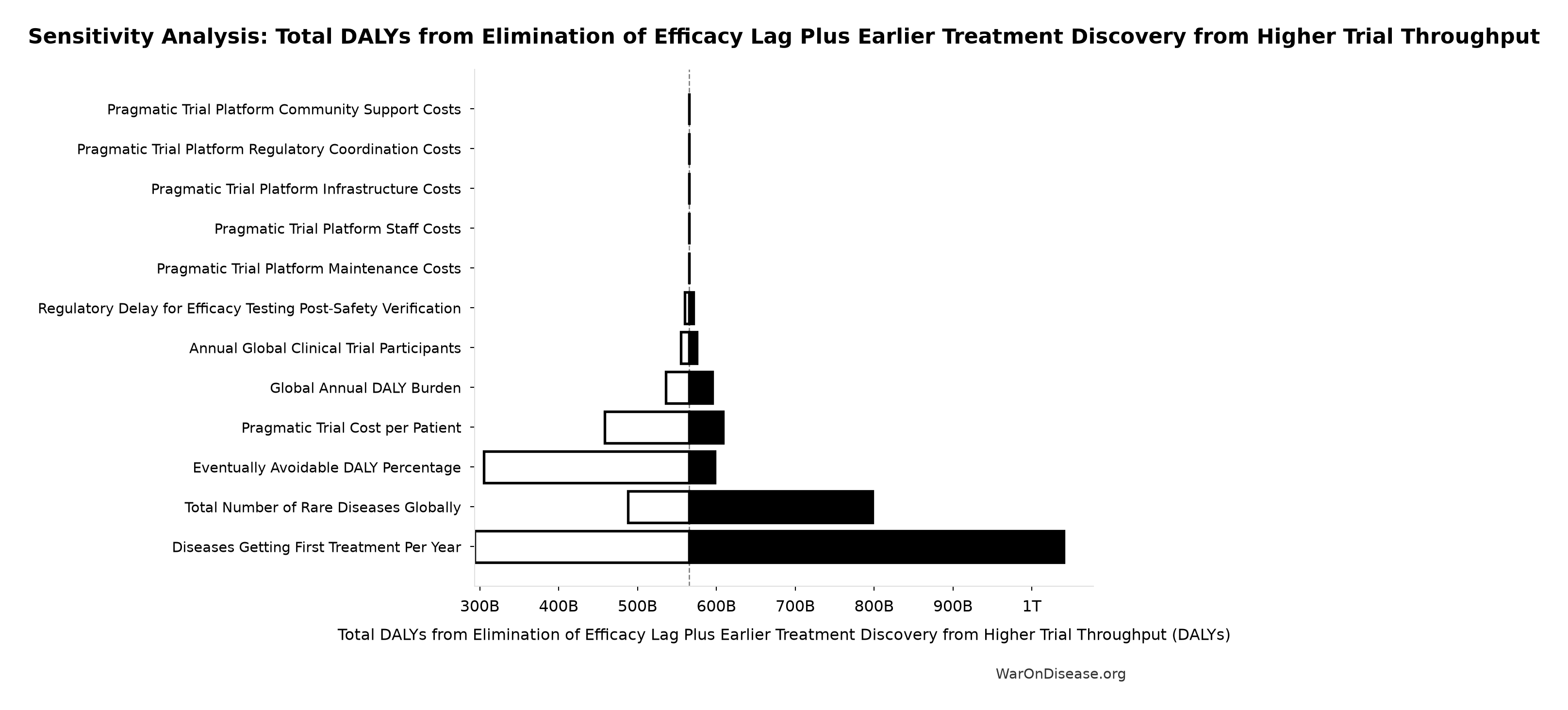
Sensitivity Indices for Total DALYs from Elimination of Efficacy Lag Plus Earlier Treatment Discovery from Higher Trial Throughput
Regression-based sensitivity showing which inputs explain the most variance in the output.
| Input Parameter | Sensitivity Coefficient | Interpretation |
|---|---|---|
| Average Total Treatment Timeline Shift (years) | 0.9320 | Strong driver |
| Eventually Avoidable DALY Percentage (percentage) | 0.3151 | Moderate driver |
| Global Annual DALY Burden (DALYs/year) | 0.1348 | Weak driver |
Interpretation: Standardized coefficients show the change in output (in SD units) per 1 SD change in input. Values near ±1 indicate strong influence; values exceeding ±1 may occur with correlated inputs.
Monte Carlo Distribution
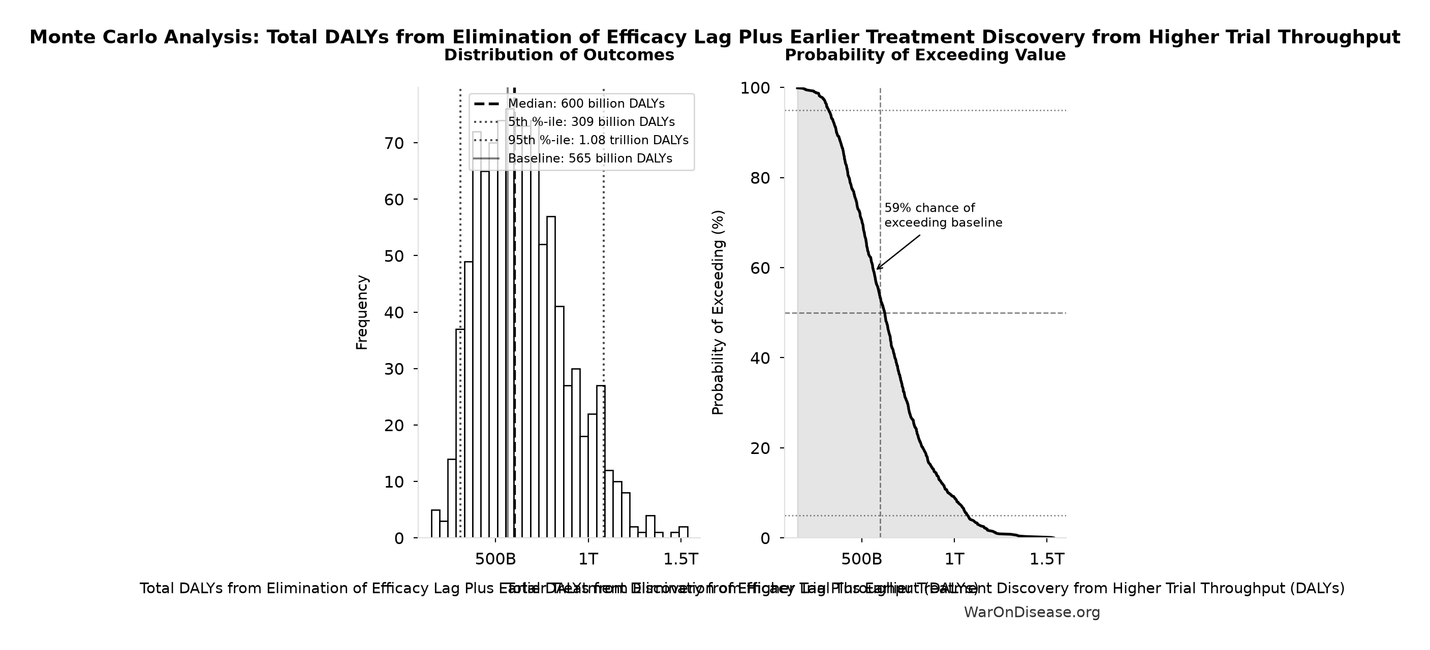
Simulation Results Summary: Total DALYs from Elimination of Efficacy Lag Plus Earlier Treatment Discovery from Higher Trial Throughput
| Statistic | Value |
|---|---|
| Baseline (deterministic) | 565 billion |
| Mean (expected value) | 635 billion |
| Median (50th percentile) | 600 billion |
| Standard Deviation | 237 billion |
| 90% Range (5th-95th percentile) | [309 billion, 1.08 trillion] |
The histogram shows 1,000 of the 10,000 Monte Carlo draws for Total DALYs from Elimination of Efficacy Lag Plus Earlier Treatment Discovery from Higher Trial Throughput; the summary statistics use all 10,000. The exceedance curve (right) shows the probability of the outcome exceeding any given value.
Exceedance Probability
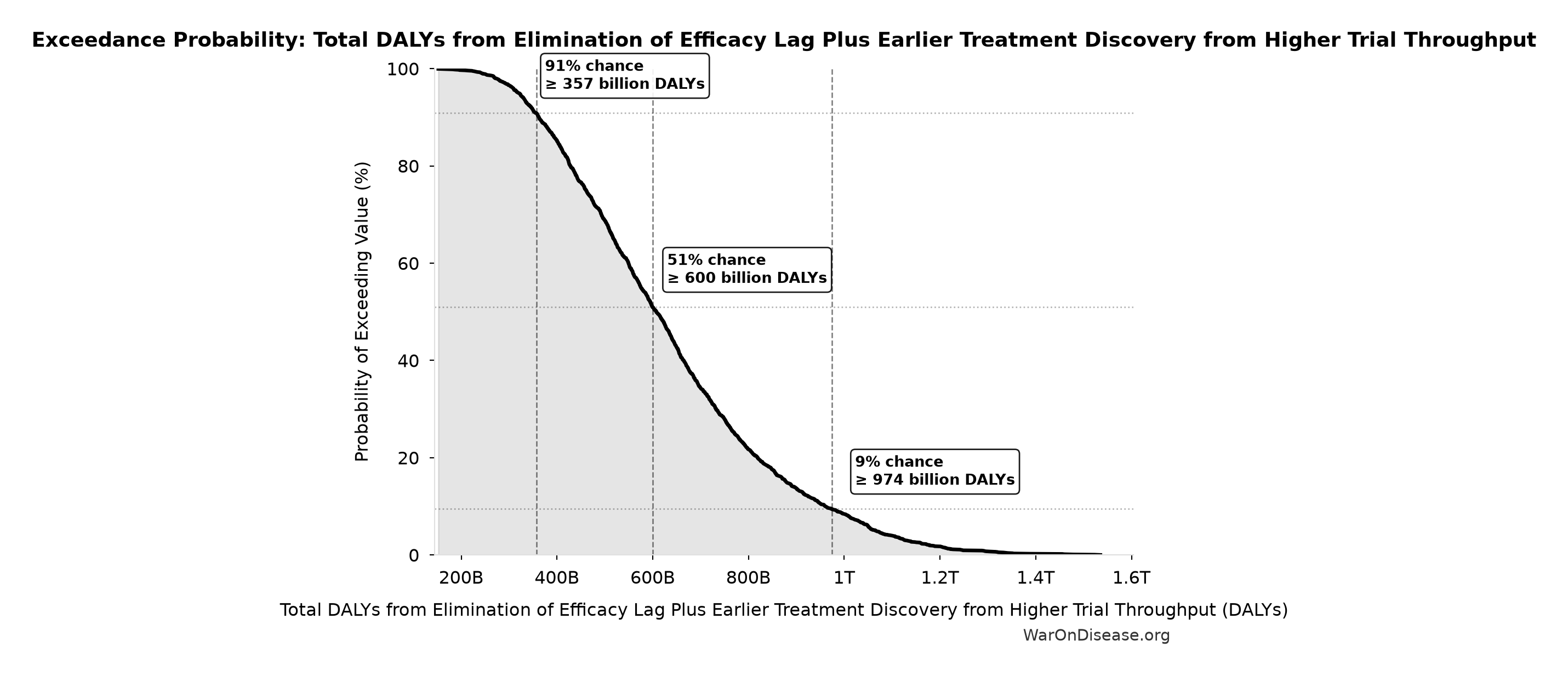
This exceedance probability chart shows the likelihood that Total DALYs from Elimination of Efficacy Lag Plus Earlier Treatment Discovery from Higher Trial Throughput will exceed any given threshold. The higher the curve at a threshold, the more likely the value exceeds it.
Total Economic Benefit from Elimination of Efficacy Lag Plus Earlier Treatment Discovery from Higher Trial Throughput: $84.8 quadrillion
Note📊 Details
Total economic value from the combined treatment timeline shift. DALYs valued at standard economic rate.
Inputs:
- Total DALYs from Elimination of Efficacy Lag Plus Earlier Treatment Discovery from Higher Trial Throughput 🔢: 565 billion DALYs
- Standard Economic Value per QALY 📊: $150,000 (SE: ±$30,000)
\[ \begin{gathered} Value_{max} \\ = DALYs_{max} \times Value_{QALY} \\ = 565B \times \$150K \\ = \$84800T \end{gathered} \] where: \[ \begin{gathered} DALYs_{max} \\ = DALYs_{global,ann} \times Pct_{avoid,DALY} \times T_{accel,max} \\ = 2.88B \times 92.6\% \times 212 \\ = 565B \end{gathered} \] where: \[ T_{accel,max} = T_{accel} + T_{lag} = 204 + 8.2 = 212 \] where: \[ \begin{gathered} T_{accel} \\ = T_{first,SQ} \times \left(1 - \frac{1}{k_{capacity}}\right) \\ = 222 \times \left(1 - \frac{1}{12.3}\right) \\ = 204 \end{gathered} \] where: \[ \begin{gathered} T_{first,SQ} \\ = T_{queue,SQ} \times 0.5 \\ = 443 \times 0.5 \\ = 222 \end{gathered} \] where: \[ \begin{gathered} T_{queue,SQ} \\ = \frac{N_{untreated}}{Treatments_{new,ann}} \\ = \frac{6{,}650}{15} \\ = 443 \end{gathered} \] where: \[ \begin{gathered} N_{untreated} \\ = N_{rare} \times 0.95 \\ = 7{,}000 \times 0.95 \\ = 6{,}650 \end{gathered} \] where: \[ \begin{gathered} k_{capacity} \\ = \frac{N_{fundable,ref}}{Slots_{curr}} \\ = \frac{23.4M}{1.9M} \\ = 12.3 \end{gathered} \] where: \[ \begin{gathered} N_{fundable,ref} \\ = \frac{Subsidies_{trial,ref}}{Cost_{pragmatic,pt}} \\ = \frac{\$21.8B}{\$929} \\ = 23.4M \end{gathered} \] where: \[ \begin{gathered} Subsidies_{trial,ref} \\ = Funding_{trial,ref} - OPEX_{trial} \\ = \$21.8B - \$40M \\ = \$21.8B \end{gathered} \] where: \[ \begin{gathered} OPEX_{trial} \\ = Cost_{platform} + Cost_{staff} + Cost_{infra} \\ + Cost_{regulatory} + Cost_{community} \\ = \$15M + \$10M + \$8M + \$5M + \$2M \\ = \$40M \end{gathered} \] ? Low confidence
Sensitivity Analysis
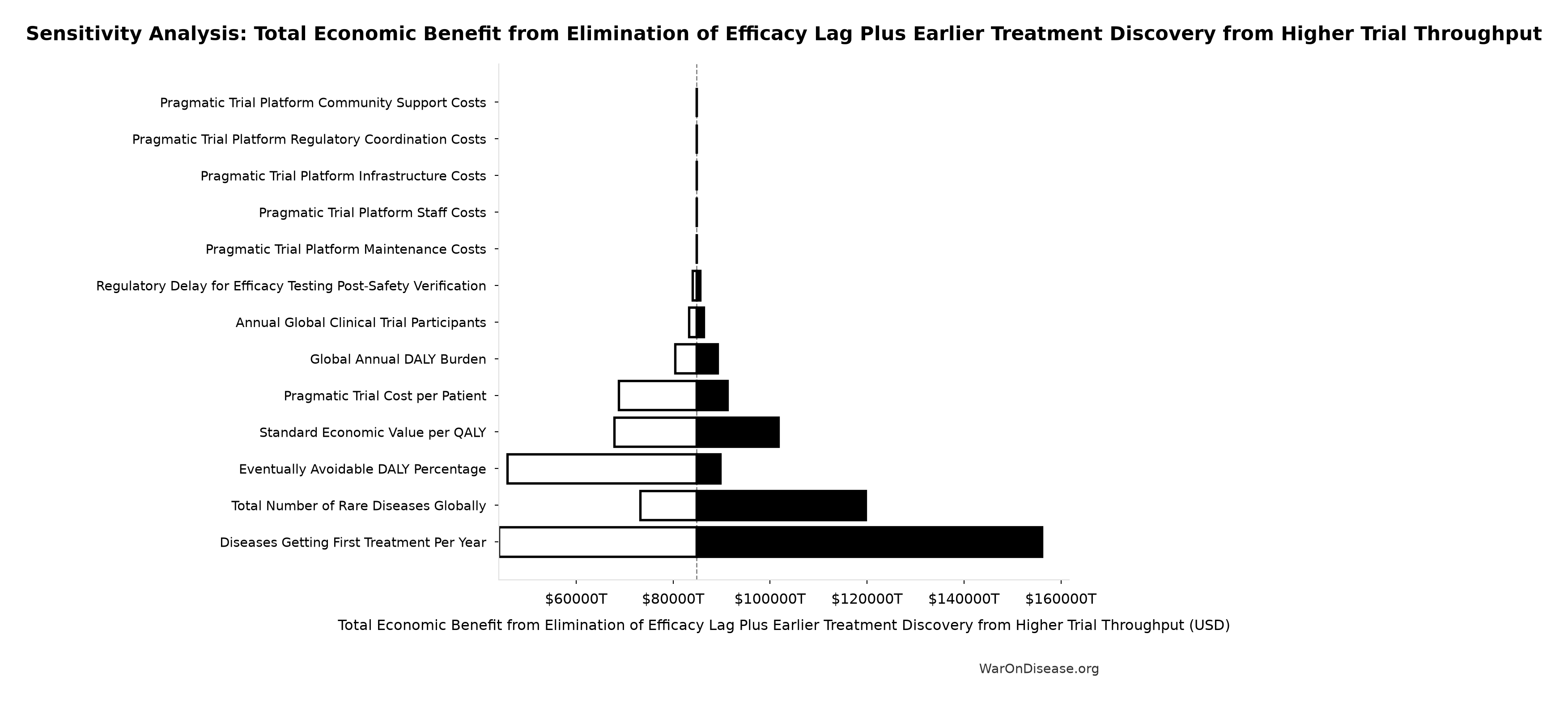
Sensitivity Indices for Total Economic Benefit from Elimination of Efficacy Lag Plus Earlier Treatment Discovery from Higher Trial Throughput
Regression-based sensitivity showing which inputs explain the most variance in the output.
| Input Parameter | Sensitivity Coefficient | Interpretation |
|---|---|---|
| Total DALYs from Elimination of Efficacy Lag Plus Earlier Treatment Discovery from Higher Trial Throughput (DALYs) | 0.8856 | Strong driver |
| Standard Economic Value per QALY (USD/QALY) | 0.4321 | Moderate driver |
Interpretation: Standardized coefficients show the change in output (in SD units) per 1 SD change in input. Values near ±1 indicate strong influence; values exceeding ±1 may occur with correlated inputs.
Monte Carlo Distribution
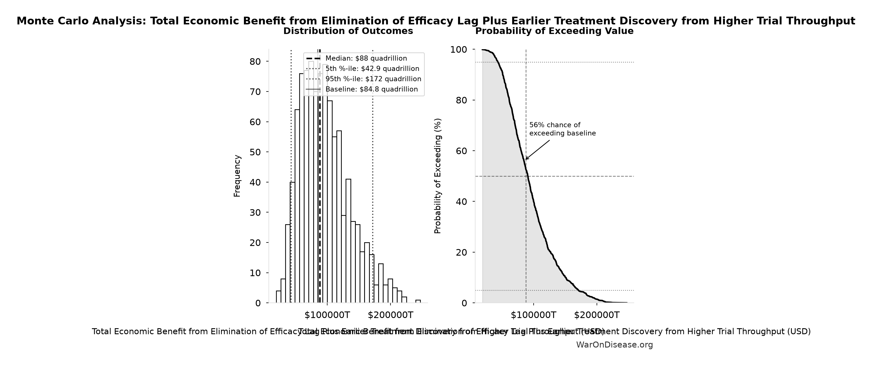
Simulation Results Summary: Total Economic Benefit from Elimination of Efficacy Lag Plus Earlier Treatment Discovery from Higher Trial Throughput
| Statistic | Value |
|---|---|
| Baseline (deterministic) | $84.8 quadrillion |
| Mean (expected value) | $95 quadrillion |
| Median (50th percentile) | $88 quadrillion |
| Standard Deviation | $40.2 quadrillion |
| 90% Range (5th-95th percentile) | [$42.9 quadrillion, $172 quadrillion] |
The histogram shows 1,000 of the 10,000 Monte Carlo draws for Total Economic Benefit from Elimination of Efficacy Lag Plus Earlier Treatment Discovery from Higher Trial Throughput; the summary statistics use all 10,000. The exceedance curve (right) shows the probability of the outcome exceeding any given value.
Exceedance Probability
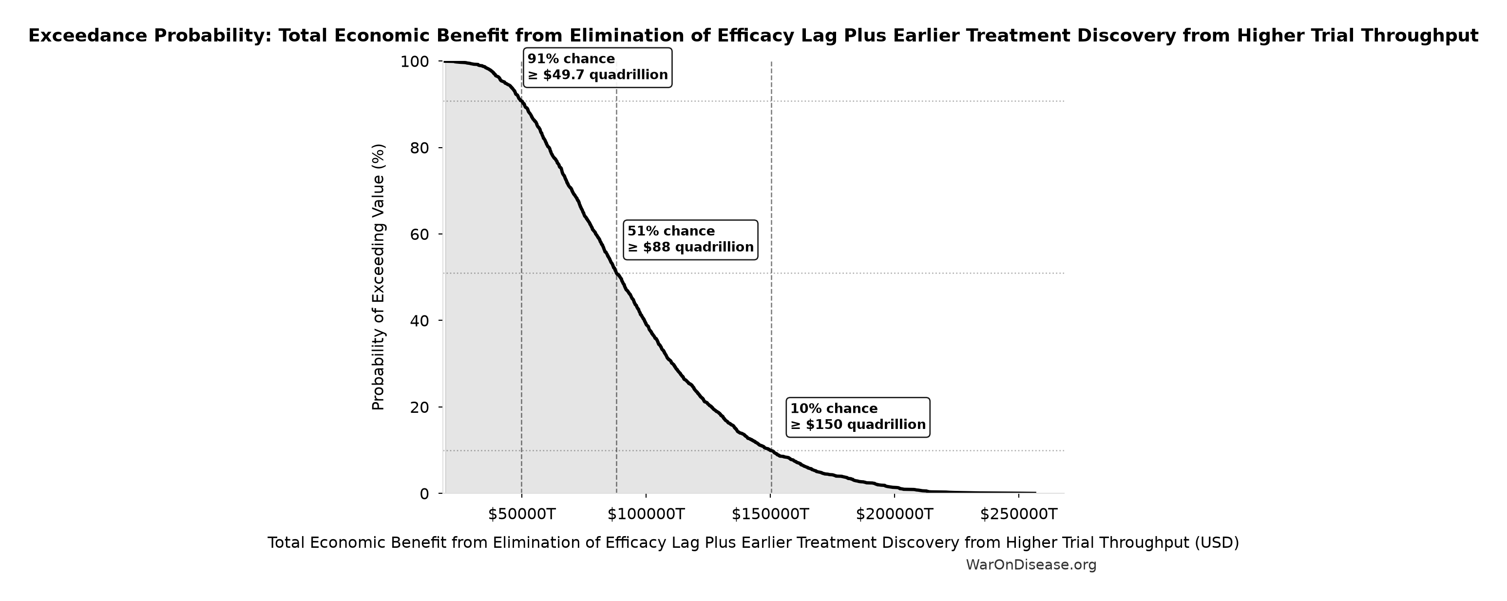
This exceedance probability chart shows the likelihood that Total Economic Benefit from Elimination of Efficacy Lag Plus Earlier Treatment Discovery from Higher Trial Throughput will exceed any given threshold. The higher the curve at a threshold, the more likely the value exceeds it.
Total Lives Saved from Elimination of Efficacy Lag Plus Earlier Treatment Discovery from Higher Trial Throughput: 10.7 billion deaths
Note📊 Details
Total eventually avoidable deaths from the combined treatment timeline shift. Represents deaths prevented when cures arrive earlier due to both increased trial capacity and eliminated efficacy lag.
Inputs:
- Global Daily Deaths from Disease and Aging 📊: 150 thousand deaths/day (SE: ±7,500 deaths/day)
- Average Total Treatment Timeline Shift 🔢: 212 years
\[ \begin{gathered} Lives_{max} \\ = Deaths_{disease,daily} \times T_{accel,max} \times 338 \\ = 150{,}000 \times 212 \times 338 \\ = 10.7B \end{gathered} \] where: \[ T_{accel,max} = T_{accel} + T_{lag} = 204 + 8.2 = 212 \] where: \[ \begin{gathered} T_{accel} \\ = T_{first,SQ} \times \left(1 - \frac{1}{k_{capacity}}\right) \\ = 222 \times \left(1 - \frac{1}{12.3}\right) \\ = 204 \end{gathered} \] where: \[ \begin{gathered} T_{first,SQ} \\ = T_{queue,SQ} \times 0.5 \\ = 443 \times 0.5 \\ = 222 \end{gathered} \] where: \[ \begin{gathered} T_{queue,SQ} \\ = \frac{N_{untreated}}{Treatments_{new,ann}} \\ = \frac{6{,}650}{15} \\ = 443 \end{gathered} \] where: \[ \begin{gathered} N_{untreated} \\ = N_{rare} \times 0.95 \\ = 7{,}000 \times 0.95 \\ = 6{,}650 \end{gathered} \] where: \[ \begin{gathered} k_{capacity} \\ = \frac{N_{fundable,ref}}{Slots_{curr}} \\ = \frac{23.4M}{1.9M} \\ = 12.3 \end{gathered} \] where: \[ \begin{gathered} N_{fundable,ref} \\ = \frac{Subsidies_{trial,ref}}{Cost_{pragmatic,pt}} \\ = \frac{\$21.8B}{\$929} \\ = 23.4M \end{gathered} \] where: \[ \begin{gathered} Subsidies_{trial,ref} \\ = Funding_{trial,ref} - OPEX_{trial} \\ = \$21.8B - \$40M \\ = \$21.8B \end{gathered} \] where: \[ \begin{gathered} OPEX_{trial} \\ = Cost_{platform} + Cost_{staff} + Cost_{infra} \\ + Cost_{regulatory} + Cost_{community} \\ = \$15M + \$10M + \$8M + \$5M + \$2M \\ = \$40M \end{gathered} \] ? Low confidence
Sensitivity Analysis
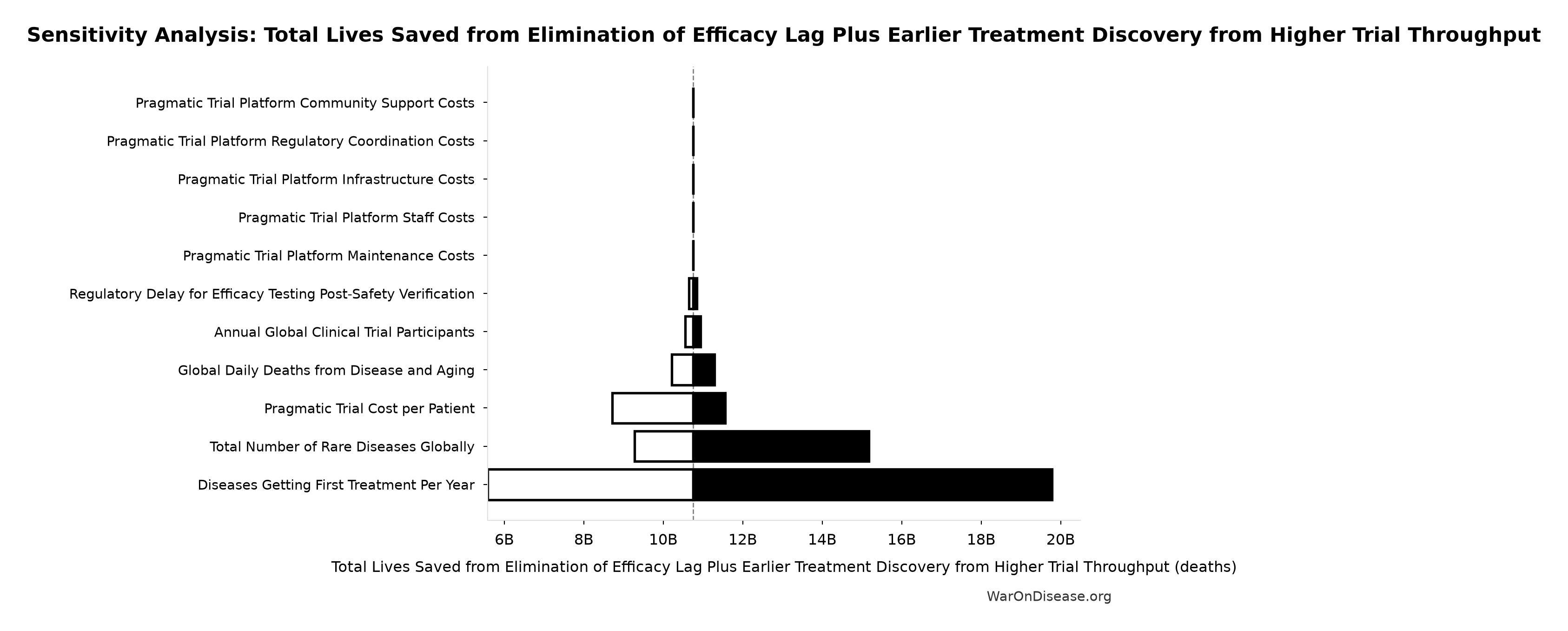
Sensitivity Indices for Total Lives Saved from Elimination of Efficacy Lag Plus Earlier Treatment Discovery from Higher Trial Throughput
Regression-based sensitivity showing which inputs explain the most variance in the output.
| Input Parameter | Sensitivity Coefficient | Interpretation |
|---|---|---|
| Average Total Treatment Timeline Shift (years) | 0.9886 | Strong driver |
| Global Daily Deaths from Disease and Aging (deaths/day) | 0.1418 | Weak driver |
Interpretation: Standardized coefficients show the change in output (in SD units) per 1 SD change in input. Values near ±1 indicate strong influence; values exceeding ±1 may occur with correlated inputs.
Monte Carlo Distribution
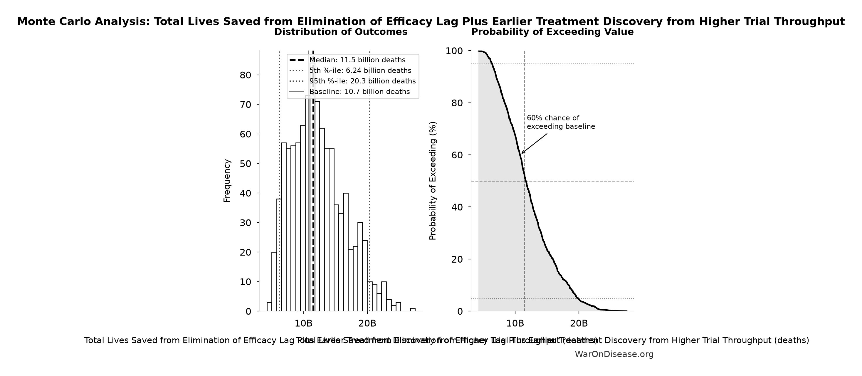
Simulation Results Summary: Total Lives Saved from Elimination of Efficacy Lag Plus Earlier Treatment Discovery from Higher Trial Throughput
| Statistic | Value |
|---|---|
| Baseline (deterministic) | 10.7 billion |
| Mean (expected value) | 12.1 billion |
| Median (50th percentile) | 11.5 billion |
| Standard Deviation | 4.28 billion |
| 90% Range (5th-95th percentile) | [6.24 billion, 20.3 billion] |
The histogram shows 1,000 of the 10,000 Monte Carlo draws for Total Lives Saved from Elimination of Efficacy Lag Plus Earlier Treatment Discovery from Higher Trial Throughput; the summary statistics use all 10,000. The exceedance curve (right) shows the probability of the outcome exceeding any given value.
Exceedance Probability
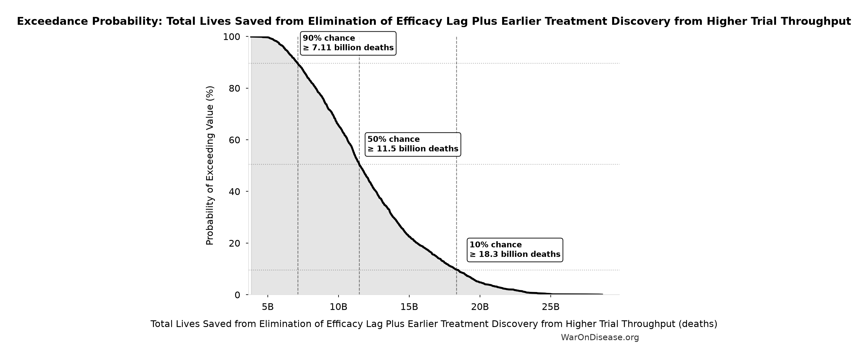
This exceedance probability chart shows the likelihood that Total Lives Saved from Elimination of Efficacy Lag Plus Earlier Treatment Discovery from Higher Trial Throughput will exceed any given threshold. The higher the curve at a threshold, the more likely the value exceeds it.
Suffering Hours Eliminated from Elimination of Efficacy Lag Plus Earlier Treatment Discovery from Higher Trial Throughput: 1.93 quadrillion hours
Note📊 Details
Hours of suffering eliminated from the combined treatment timeline shift. Calculated from YLD component of DALYs (39% of total DALYs × hours per year). One-time benefit, not annual recurring.
Inputs:
- Total DALYs from Elimination of Efficacy Lag Plus Earlier Treatment Discovery from Higher Trial Throughput 🔢: 565 billion DALYs
- YLD Proportion of Total DALYs 📊: 0.39 proportion (SE: ±0.03 proportion)
\[ \begin{gathered} Hours_{suffer,max} \\ = DALYs_{max} \times Pct_{YLD} \times 8760 \\ = 565B \times 0.39 \times 8760 \\ = 1930T \end{gathered} \] where: \[ \begin{gathered} DALYs_{max} \\ = DALYs_{global,ann} \times Pct_{avoid,DALY} \times T_{accel,max} \\ = 2.88B \times 92.6\% \times 212 \\ = 565B \end{gathered} \] where: \[ T_{accel,max} = T_{accel} + T_{lag} = 204 + 8.2 = 212 \] where: \[ \begin{gathered} T_{accel} \\ = T_{first,SQ} \times \left(1 - \frac{1}{k_{capacity}}\right) \\ = 222 \times \left(1 - \frac{1}{12.3}\right) \\ = 204 \end{gathered} \] where: \[ \begin{gathered} T_{first,SQ} \\ = T_{queue,SQ} \times 0.5 \\ = 443 \times 0.5 \\ = 222 \end{gathered} \] where: \[ \begin{gathered} T_{queue,SQ} \\ = \frac{N_{untreated}}{Treatments_{new,ann}} \\ = \frac{6{,}650}{15} \\ = 443 \end{gathered} \] where: \[ \begin{gathered} N_{untreated} \\ = N_{rare} \times 0.95 \\ = 7{,}000 \times 0.95 \\ = 6{,}650 \end{gathered} \] where: \[ \begin{gathered} k_{capacity} \\ = \frac{N_{fundable,ref}}{Slots_{curr}} \\ = \frac{23.4M}{1.9M} \\ = 12.3 \end{gathered} \] where: \[ \begin{gathered} N_{fundable,ref} \\ = \frac{Subsidies_{trial,ref}}{Cost_{pragmatic,pt}} \\ = \frac{\$21.8B}{\$929} \\ = 23.4M \end{gathered} \] where: \[ \begin{gathered} Subsidies_{trial,ref} \\ = Funding_{trial,ref} - OPEX_{trial} \\ = \$21.8B - \$40M \\ = \$21.8B \end{gathered} \] where: \[ \begin{gathered} OPEX_{trial} \\ = Cost_{platform} + Cost_{staff} + Cost_{infra} \\ + Cost_{regulatory} + Cost_{community} \\ = \$15M + \$10M + \$8M + \$5M + \$2M \\ = \$40M \end{gathered} \] ? Low confidence
Sensitivity Analysis
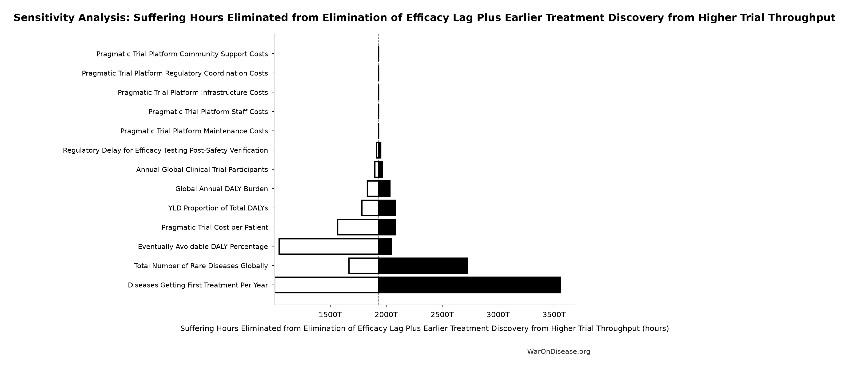
Sensitivity Indices for Suffering Hours Eliminated from Elimination of Efficacy Lag Plus Earlier Treatment Discovery from Higher Trial Throughput
Regression-based sensitivity showing which inputs explain the most variance in the output.
| Input Parameter | Sensitivity Coefficient | Interpretation |
|---|---|---|
| Total DALYs from Elimination of Efficacy Lag Plus Earlier Treatment Discovery from Higher Trial Throughput (DALYs) | 0.9776 | Strong driver |
| YLD Proportion of Total DALYs (proportion) | 0.2007 | Weak driver |
Interpretation: Standardized coefficients show the change in output (in SD units) per 1 SD change in input. Values near ±1 indicate strong influence; values exceeding ±1 may occur with correlated inputs.
Monte Carlo Distribution
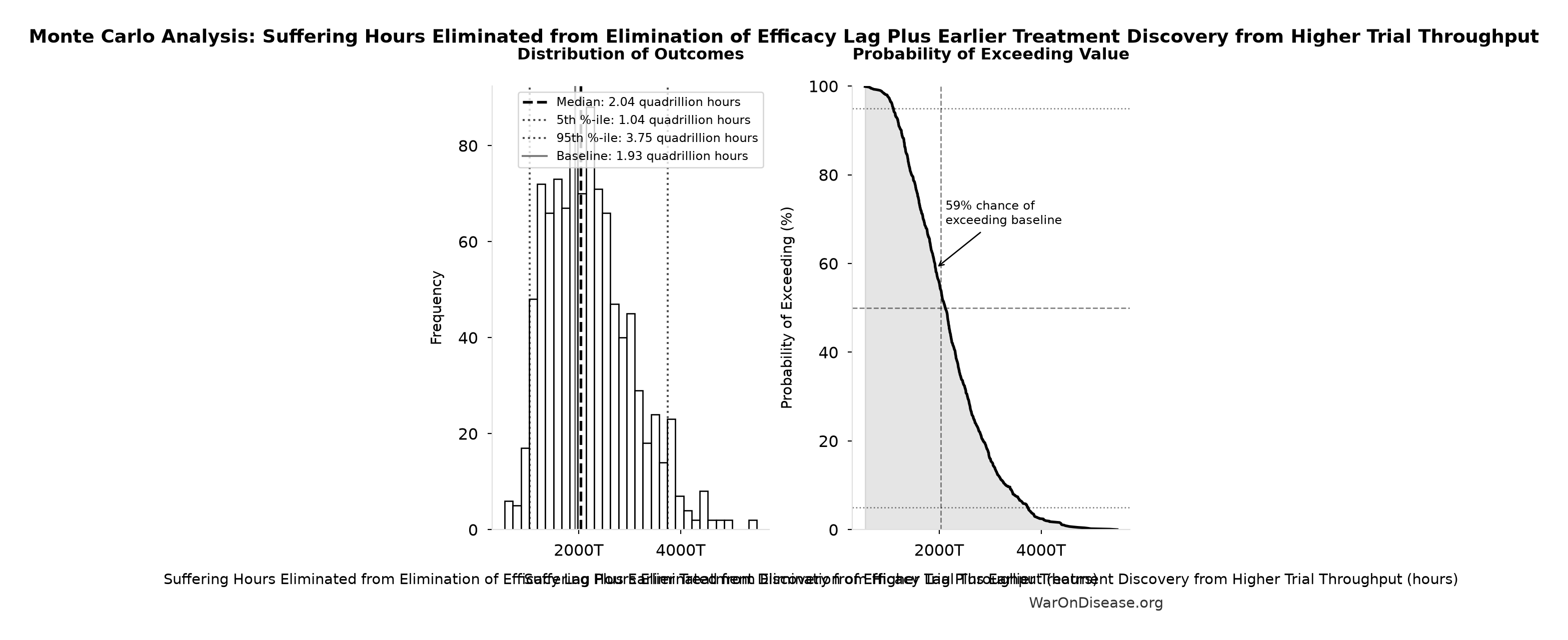
Simulation Results Summary: Suffering Hours Eliminated from Elimination of Efficacy Lag Plus Earlier Treatment Discovery from Higher Trial Throughput
| Statistic | Value |
|---|---|
| Baseline (deterministic) | 1.93 quadrillion |
| Mean (expected value) | 2.17 quadrillion |
| Median (50th percentile) | 2.04 quadrillion |
| Standard Deviation | 828 trillion |
| 90% Range (5th-95th percentile) | [1.04 quadrillion, 3.75 quadrillion] |
The histogram shows 1,000 of the 10,000 Monte Carlo draws for Suffering Hours Eliminated from Elimination of Efficacy Lag Plus Earlier Treatment Discovery from Higher Trial Throughput; the summary statistics use all 10,000. The exceedance curve (right) shows the probability of the outcome exceeding any given value.
Exceedance Probability
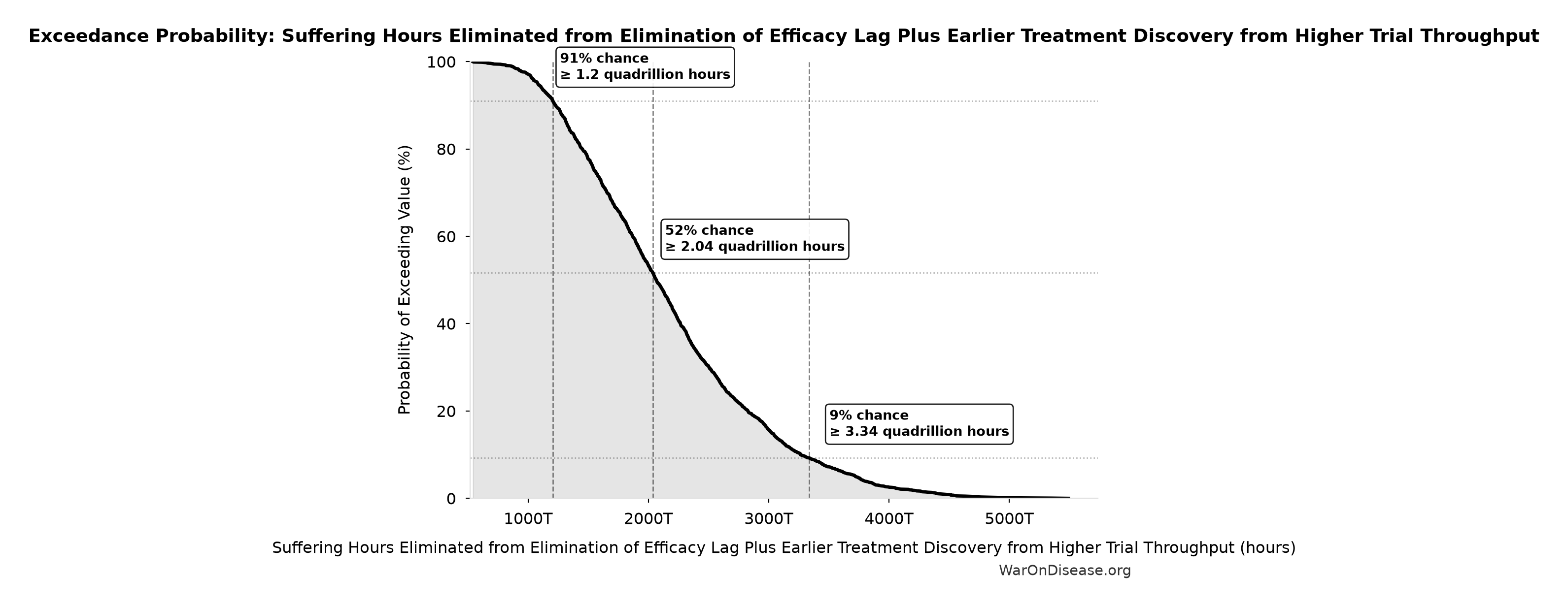
This exceedance probability chart shows the likelihood that Suffering Hours Eliminated from Elimination of Efficacy Lag Plus Earlier Treatment Discovery from Higher Trial Throughput will exceed any given threshold. The higher the curve at a threshold, the more likely the value exceeds it.
Average Total Treatment Timeline Shift: 212 years
Note📊 Details
Average years earlier patients receive treatments from increased pragmatic trial capacity plus efficacy lag elimination for treatments already discovered.
Inputs:
- Treatment Timeline Acceleration from Pragmatic Trial Capacity 🔢: 204 years
- Regulatory Delay for Efficacy Testing Post-Safety Verification 📊: 8.2 years (SE: ±2 years)
\[ T_{accel,max} = T_{accel} + T_{lag} = 204 + 8.2 = 212 \] where: \[ \begin{gathered} T_{accel} \\ = T_{first,SQ} \times \left(1 - \frac{1}{k_{capacity}}\right) \\ = 222 \times \left(1 - \frac{1}{12.3}\right) \\ = 204 \end{gathered} \] where: \[ \begin{gathered} T_{first,SQ} \\ = T_{queue,SQ} \times 0.5 \\ = 443 \times 0.5 \\ = 222 \end{gathered} \] where: \[ \begin{gathered} T_{queue,SQ} \\ = \frac{N_{untreated}}{Treatments_{new,ann}} \\ = \frac{6{,}650}{15} \\ = 443 \end{gathered} \] where: \[ \begin{gathered} N_{untreated} \\ = N_{rare} \times 0.95 \\ = 7{,}000 \times 0.95 \\ = 6{,}650 \end{gathered} \] where: \[ \begin{gathered} k_{capacity} \\ = \frac{N_{fundable,ref}}{Slots_{curr}} \\ = \frac{23.4M}{1.9M} \\ = 12.3 \end{gathered} \] where: \[ \begin{gathered} N_{fundable,ref} \\ = \frac{Subsidies_{trial,ref}}{Cost_{pragmatic,pt}} \\ = \frac{\$21.8B}{\$929} \\ = 23.4M \end{gathered} \] where: \[ \begin{gathered} Subsidies_{trial,ref} \\ = Funding_{trial,ref} - OPEX_{trial} \\ = \$21.8B - \$40M \\ = \$21.8B \end{gathered} \] where: \[ \begin{gathered} OPEX_{trial} \\ = Cost_{platform} + Cost_{staff} + Cost_{infra} \\ + Cost_{regulatory} + Cost_{community} \\ = \$15M + \$10M + \$8M + \$5M + \$2M \\ = \$40M \end{gathered} \] ? Low confidence
Sensitivity Analysis
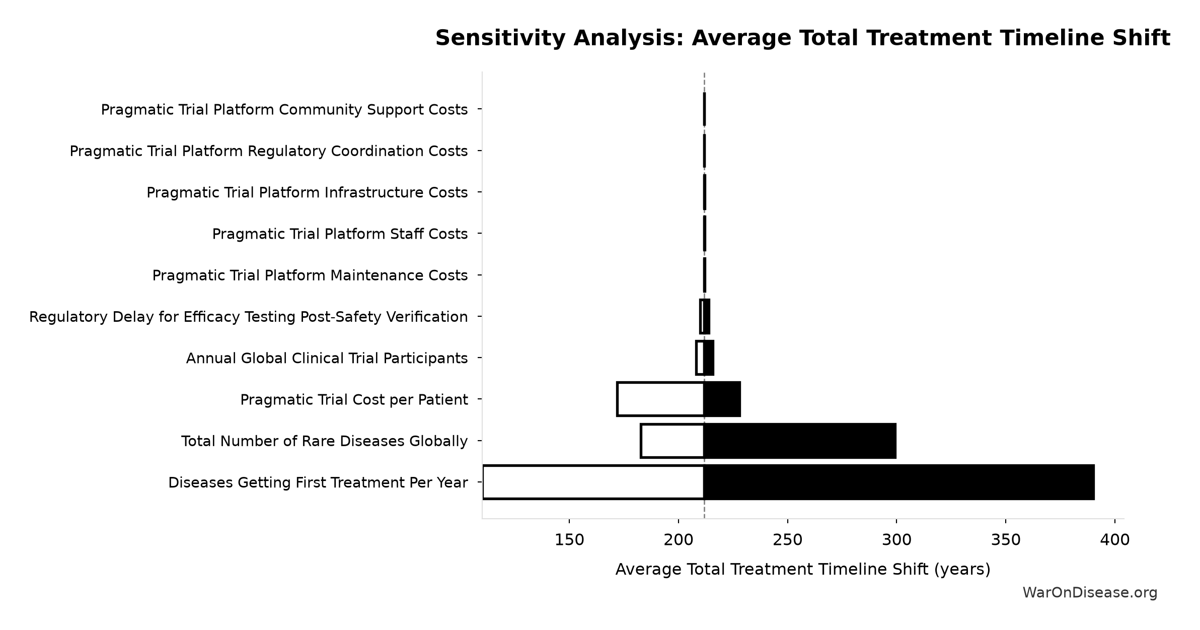
Sensitivity Indices for Average Total Treatment Timeline Shift
Regression-based sensitivity showing which inputs explain the most variance in the output.
| Input Parameter | Sensitivity Coefficient | Interpretation |
|---|---|---|
| Treatment Timeline Acceleration from Pragmatic Trial Capacity (years) | 0.9998 | Strong driver |
| Regulatory Delay for Efficacy Testing Post-Safety Verification (years) | 0.0238 | Minimal effect |
Interpretation: Standardized coefficients show the change in output (in SD units) per 1 SD change in input. Values near ±1 indicate strong influence; values exceeding ±1 may occur with correlated inputs.
Monte Carlo Distribution
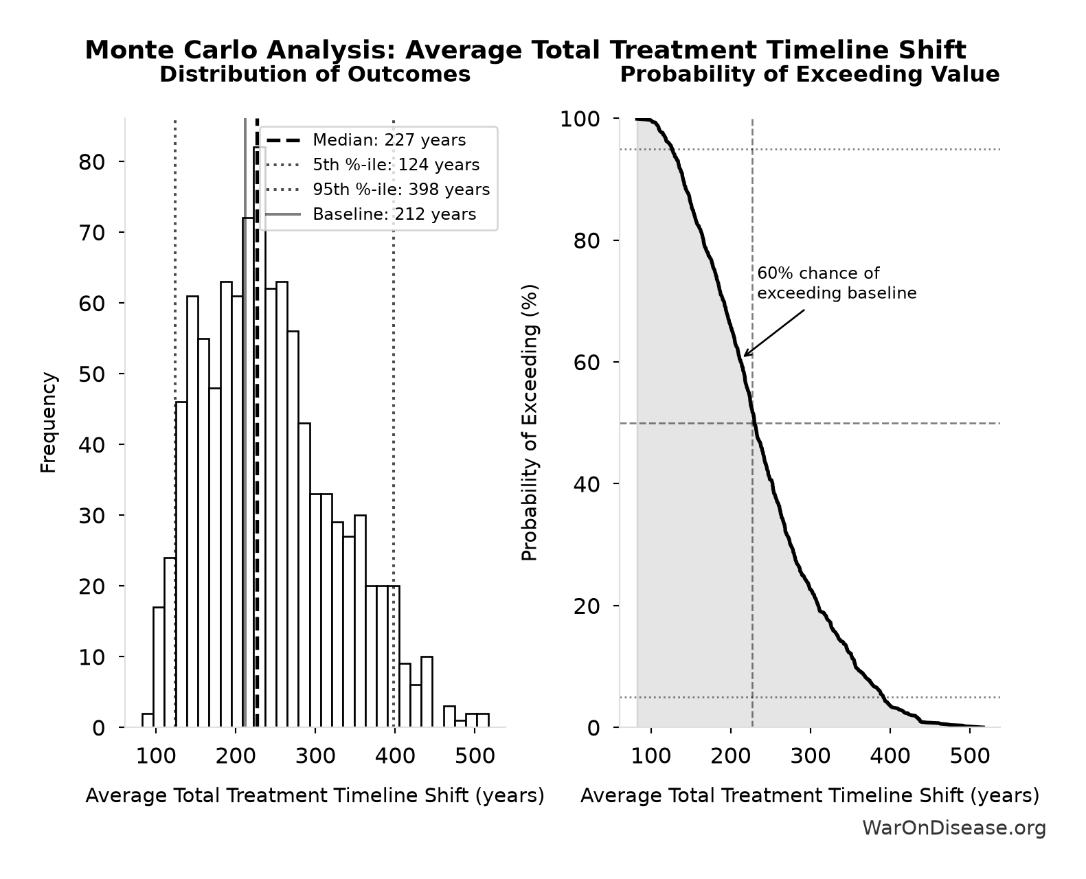
Simulation Results Summary: Average Total Treatment Timeline Shift
| Statistic | Value |
|---|---|
| Baseline (deterministic) | 212 |
| Mean (expected value) | 239 |
| Median (50th percentile) | 227 |
| Standard Deviation | 83.4 |
| 90% Range (5th-95th percentile) | [124, 398] |
The histogram shows 1,000 of the 10,000 Monte Carlo draws for Average Total Treatment Timeline Shift; the summary statistics use all 10,000. The exceedance curve (right) shows the probability of the outcome exceeding any given value.
Exceedance Probability
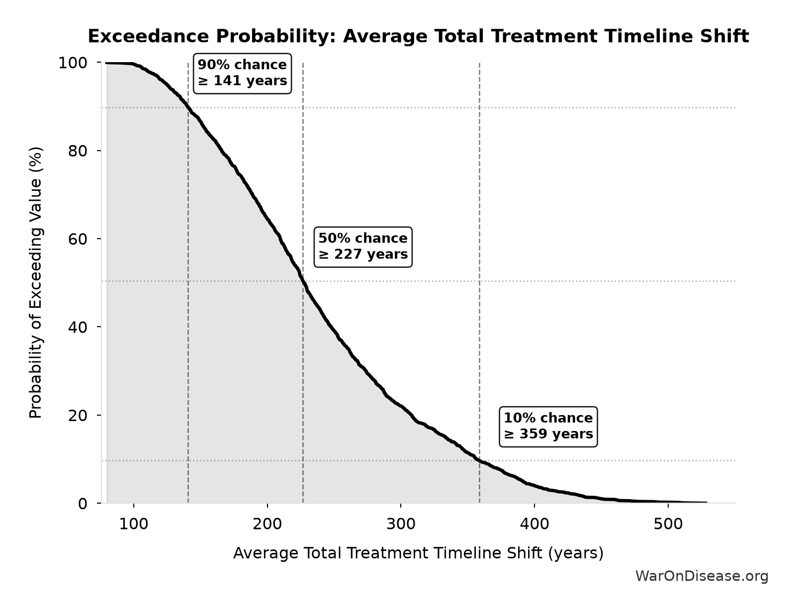
This exceedance probability chart shows the likelihood that Average Total Treatment Timeline Shift will exceed any given threshold. The higher the curve at a threshold, the more likely the value exceeds it.
Treatment Timeline Acceleration from Pragmatic Trial Capacity: 204 years
Note📊 Details
Years earlier the average first treatment arrives due to increased pragmatic trial capacity. Calculated as the status quo timeline reduced by the inverse of the capacity multiplier. Uses only trial capacity multiplier (not combined with valley of death rescue) because additional candidates do not directly speed therapeutic space exploration.
Inputs:
- Status Quo Average Years to First Treatment 🔢: 222 years
- Pragmatic Trial Capacity Multiplier at Treaty-Scale Funding 🔢: 12.3x
\[ \begin{gathered} T_{accel} \\ = T_{first,SQ} \times \left(1 - \frac{1}{k_{capacity}}\right) \\ = 222 \times \left(1 - \frac{1}{12.3}\right) \\ = 204 \end{gathered} \] where: \[ \begin{gathered} T_{first,SQ} \\ = T_{queue,SQ} \times 0.5 \\ = 443 \times 0.5 \\ = 222 \end{gathered} \] where: \[ \begin{gathered} T_{queue,SQ} \\ = \frac{N_{untreated}}{Treatments_{new,ann}} \\ = \frac{6{,}650}{15} \\ = 443 \end{gathered} \] where: \[ \begin{gathered} N_{untreated} \\ = N_{rare} \times 0.95 \\ = 7{,}000 \times 0.95 \\ = 6{,}650 \end{gathered} \] where: \[ \begin{gathered} k_{capacity} \\ = \frac{N_{fundable,ref}}{Slots_{curr}} \\ = \frac{23.4M}{1.9M} \\ = 12.3 \end{gathered} \] where: \[ \begin{gathered} N_{fundable,ref} \\ = \frac{Subsidies_{trial,ref}}{Cost_{pragmatic,pt}} \\ = \frac{\$21.8B}{\$929} \\ = 23.4M \end{gathered} \] where: \[ \begin{gathered} Subsidies_{trial,ref} \\ = Funding_{trial,ref} - OPEX_{trial} \\ = \$21.8B - \$40M \\ = \$21.8B \end{gathered} \] where: \[ \begin{gathered} OPEX_{trial} \\ = Cost_{platform} + Cost_{staff} + Cost_{infra} \\ + Cost_{regulatory} + Cost_{community} \\ = \$15M + \$10M + \$8M + \$5M + \$2M \\ = \$40M \end{gathered} \] ? Low confidence
Sensitivity Analysis
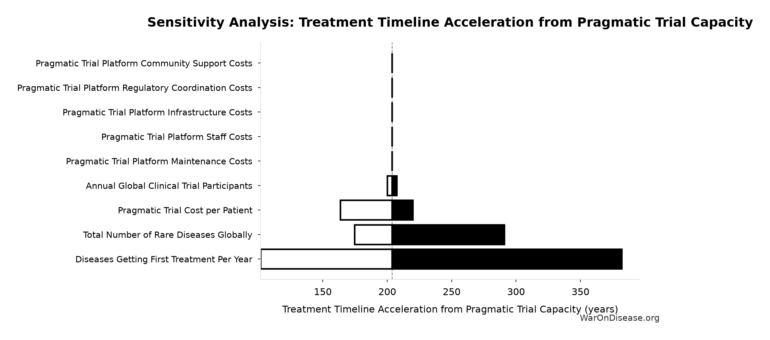
Sensitivity Indices for Treatment Timeline Acceleration from Pragmatic Trial Capacity
Regression-based sensitivity showing which inputs explain the most variance in the output.
| Input Parameter | Sensitivity Coefficient | Interpretation |
|---|---|---|
| Status Quo Average Years to First Treatment (years) | 0.9823 | Strong driver |
| Pragmatic Trial Capacity Multiplier at Treaty-Scale Funding (x) | 0.1163 | Weak driver |
Interpretation: Standardized coefficients show the change in output (in SD units) per 1 SD change in input. Values near ±1 indicate strong influence; values exceeding ±1 may occur with correlated inputs.
Monte Carlo Distribution
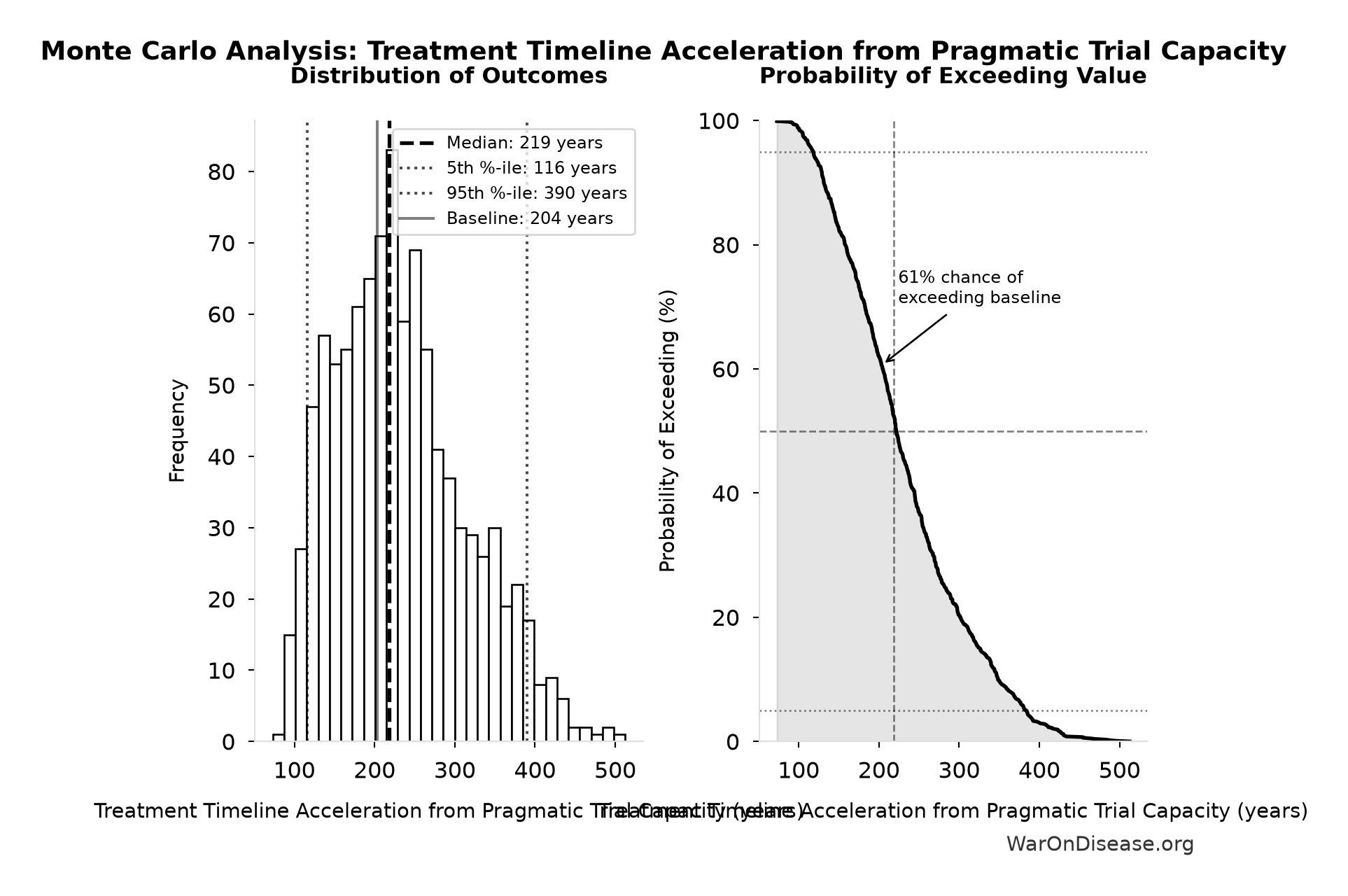
Simulation Results Summary: Treatment Timeline Acceleration from Pragmatic Trial Capacity
| Statistic | Value |
|---|---|
| Baseline (deterministic) | 204 |
| Mean (expected value) | 231 |
| Median (50th percentile) | 219 |
| Standard Deviation | 83.4 |
| 90% Range (5th-95th percentile) | [116, 390] |
The histogram shows 1,000 of the 10,000 Monte Carlo draws for Treatment Timeline Acceleration from Pragmatic Trial Capacity; the summary statistics use all 10,000. The exceedance curve (right) shows the probability of the outcome exceeding any given value.
Exceedance Probability
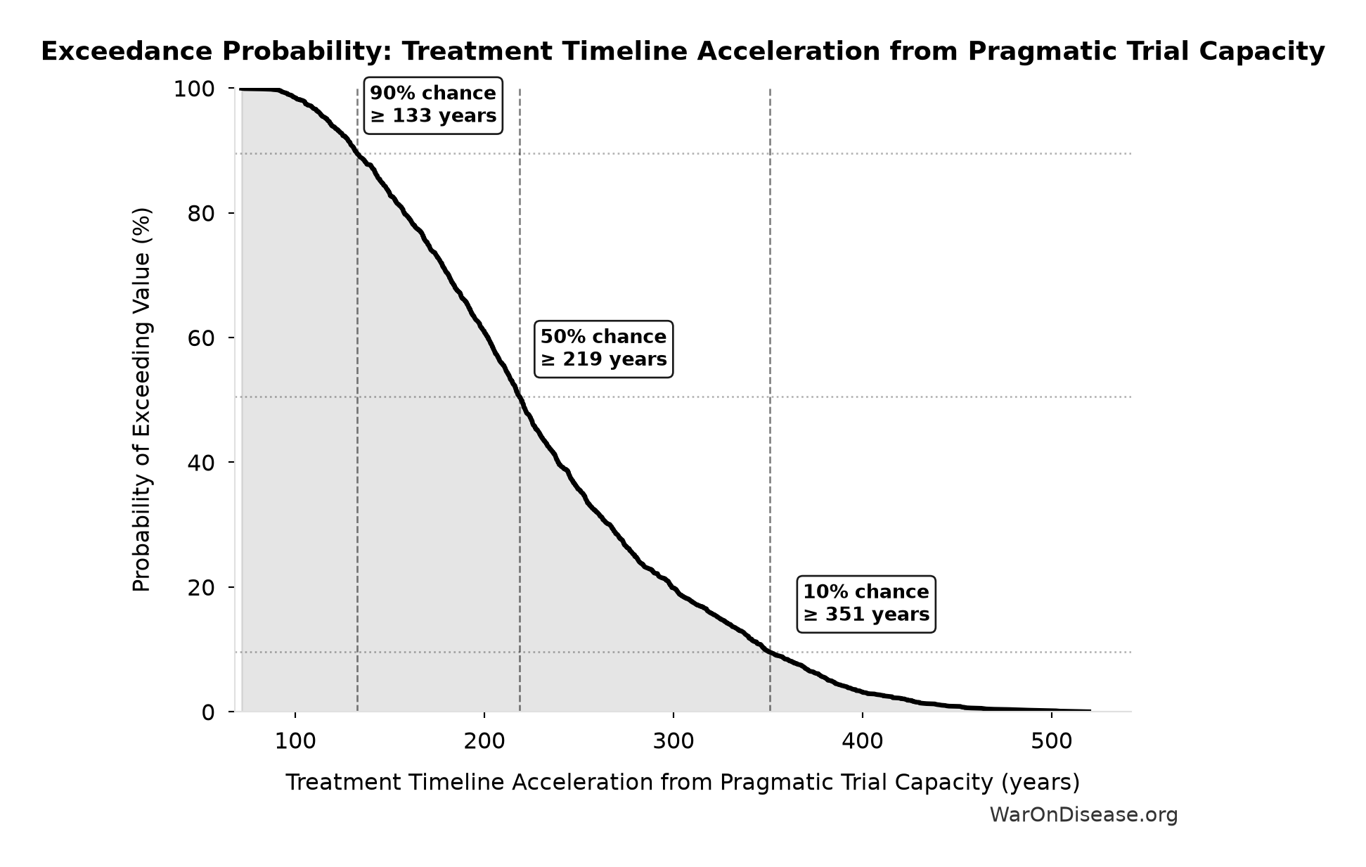
This exceedance probability chart shows the likelihood that Treatment Timeline Acceleration from Pragmatic Trial Capacity will exceed any given threshold. The higher the curve at a threshold, the more likely the value exceeds it.
Pragmatic Trial Cost Reduction Factor: 44.1x
Note📊 Details
Cost reduction factor projected for embedded pragmatic trials (traditional Phase 3 cost / pragmatic trial cost per patient)
Inputs:
- Phase 3 Cost per Patient 📊: $41,000 (95% CI: $20,000 - $120,000)
- Pragmatic Trial Cost per Patient 📊: $929 (95% CI: $97 - $3,000)
\[ \begin{gathered} k_{reduce} \\ = \frac{Cost_{P3,pt}}{Cost_{pragmatic,pt}} \\ = \frac{\$41K}{\$929} \\ = 44.1 \end{gathered} \]
✓ High confidence
Sensitivity Analysis
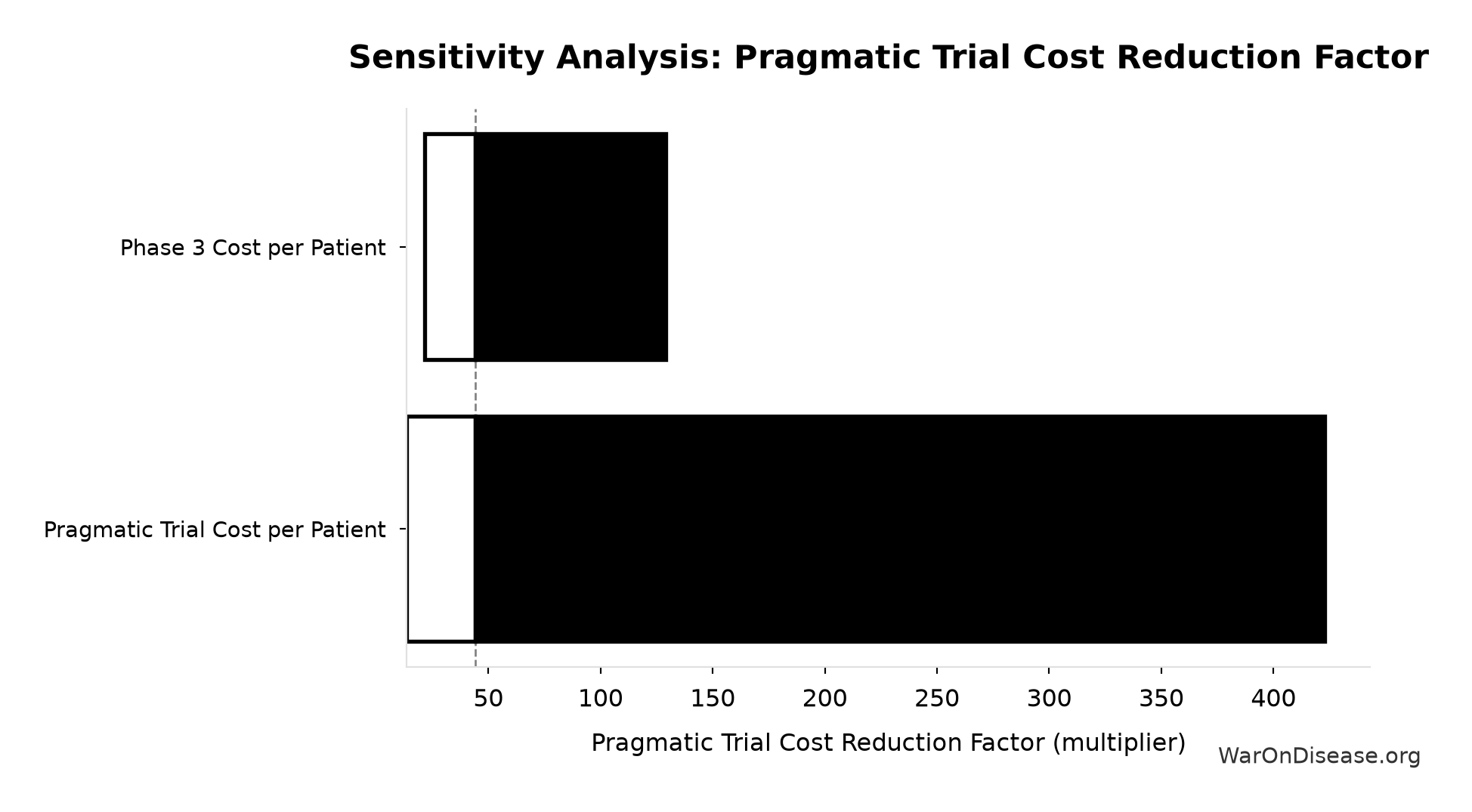
Sensitivity Indices for Pragmatic Trial Cost Reduction Factor
Regression-based sensitivity showing which inputs explain the most variance in the output.
| Input Parameter | Sensitivity Coefficient | Interpretation |
|---|---|---|
| Phase 3 Cost per Patient (USD/patient) | 0.5310 | Strong driver |
| Pragmatic Trial Cost per Patient (USD/patient) | -0.4880 | Moderate driver |
Interpretation: Standardized coefficients show the change in output (in SD units) per 1 SD change in input. Values near ±1 indicate strong influence; values exceeding ±1 may occur with correlated inputs.
Monte Carlo Distribution
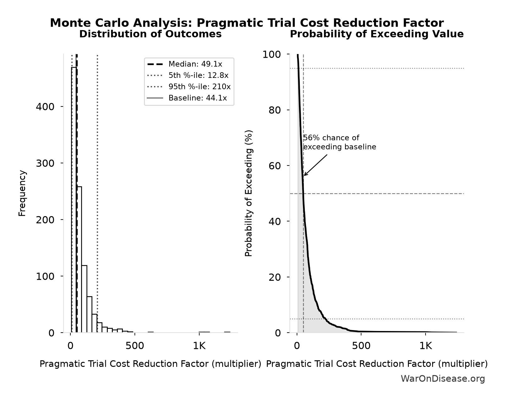
Simulation Results Summary: Pragmatic Trial Cost Reduction Factor
| Statistic | Value |
|---|---|
| Baseline (deterministic) | 44.1x |
| Mean (expected value) | 73x |
| Median (50th percentile) | 49.1x |
| Standard Deviation | 78.5x |
| 90% Range (5th-95th percentile) | [12.8x, 210x] |
The histogram shows 1,000 of the 10,000 Monte Carlo draws for Pragmatic Trial Cost Reduction Factor; the summary statistics use all 10,000. The exceedance curve (right) shows the probability of the outcome exceeding any given value.
Exceedance Probability
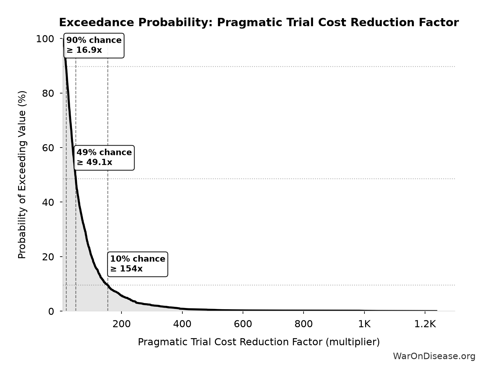
This exceedance probability chart shows the likelihood that Pragmatic Trial Cost Reduction Factor will exceed any given threshold. The higher the curve at a threshold, the more likely the value exceeds it.
Pragmatic Trial Cost Reduction Percentage: 97.7%
Note📊 Details
Trial cost reduction percentage: 1 - (pragmatic trial cost / traditional Phase 3 cost)
Inputs:
- Pragmatic Trial Cost per Patient 📊: $929 (95% CI: $97 - $3,000)
- Phase 3 Cost per Patient 📊: $41,000 (95% CI: $20,000 - $120,000)
\[ \begin{gathered} Reduce_{pct} \\ = 1 - \frac{Cost_{pragmatic,pt}}{Cost_{P3,pt}} \\ = 1 - \frac{\$929}{\$41K} \\ = 97.7\% \end{gathered} \]
✓ High confidence
Sensitivity Analysis
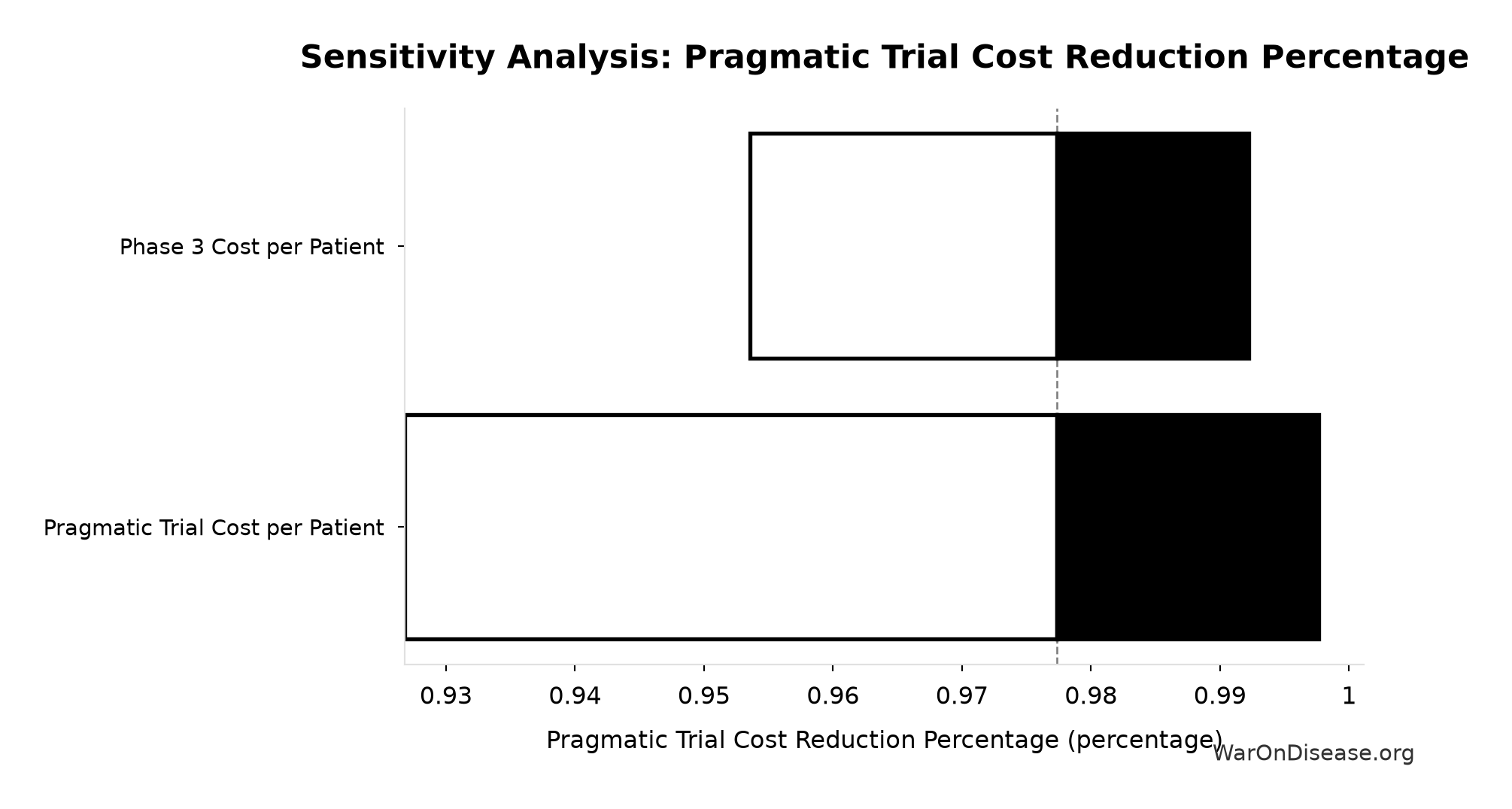
Sensitivity Indices for Pragmatic Trial Cost Reduction Percentage
Regression-based sensitivity showing which inputs explain the most variance in the output.
| Input Parameter | Sensitivity Coefficient | Interpretation |
|---|---|---|
| Pragmatic Trial Cost per Patient (USD/patient) | -0.8031 | Strong driver |
| Phase 3 Cost per Patient (USD/patient) | 0.4142 | Moderate driver |
Interpretation: Standardized coefficients show the change in output (in SD units) per 1 SD change in input. Values near ±1 indicate strong influence; values exceeding ±1 may occur with correlated inputs.
Monte Carlo Distribution
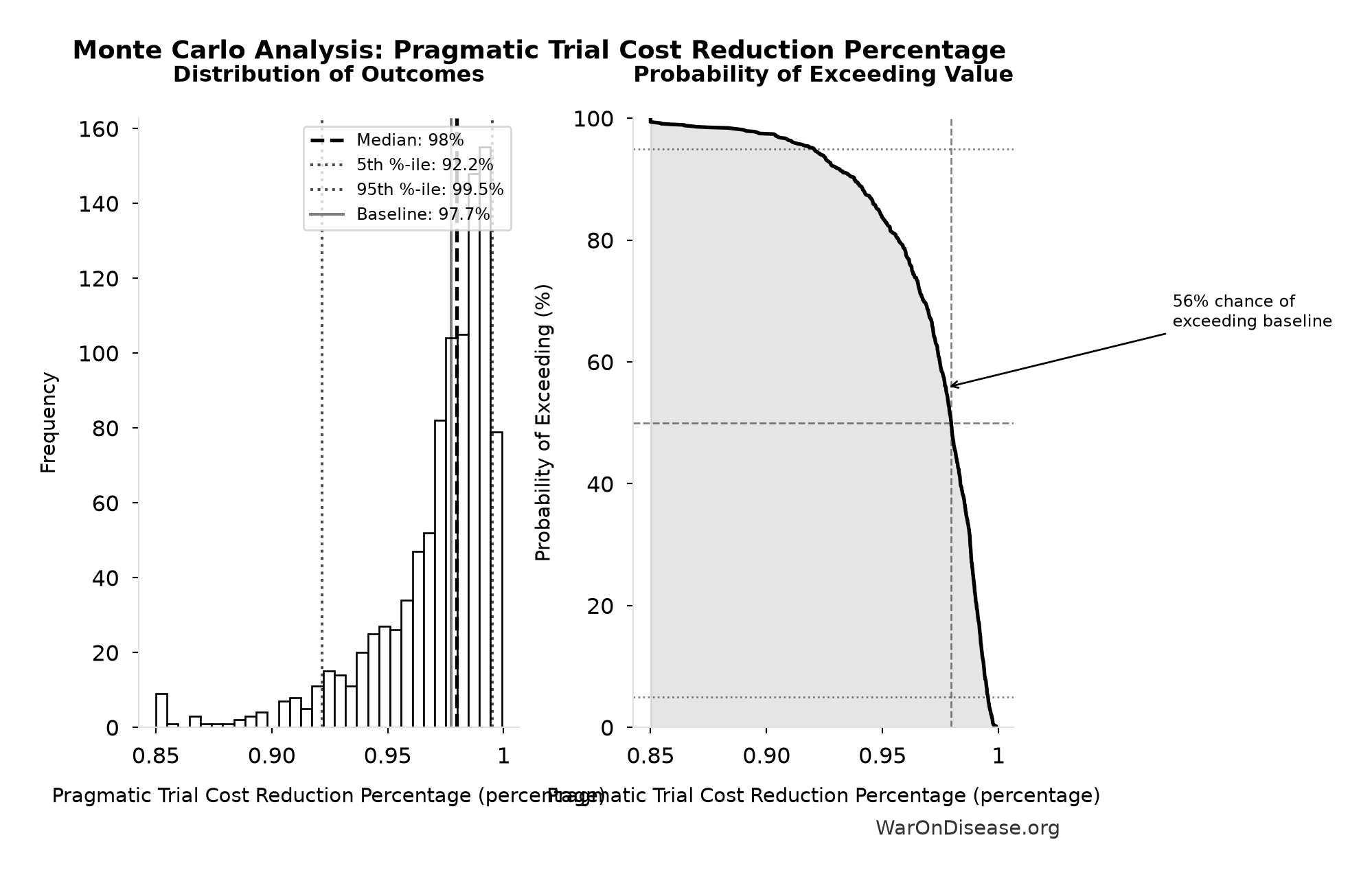
Simulation Results Summary: Pragmatic Trial Cost Reduction Percentage
| Statistic | Value |
|---|---|
| Baseline (deterministic) | 97.7% |
| Mean (expected value) | 97.2% |
| Median (50th percentile) | 98% |
| Standard Deviation | 2.48% |
| 90% Range (5th-95th percentile) | [92.2%, 99.5%] |
The histogram shows 1,000 of the 10,000 Monte Carlo draws for Pragmatic Trial Cost Reduction Percentage; the summary statistics use all 10,000. The exceedance curve (right) shows the probability of the outcome exceeding any given value.
Exceedance Probability
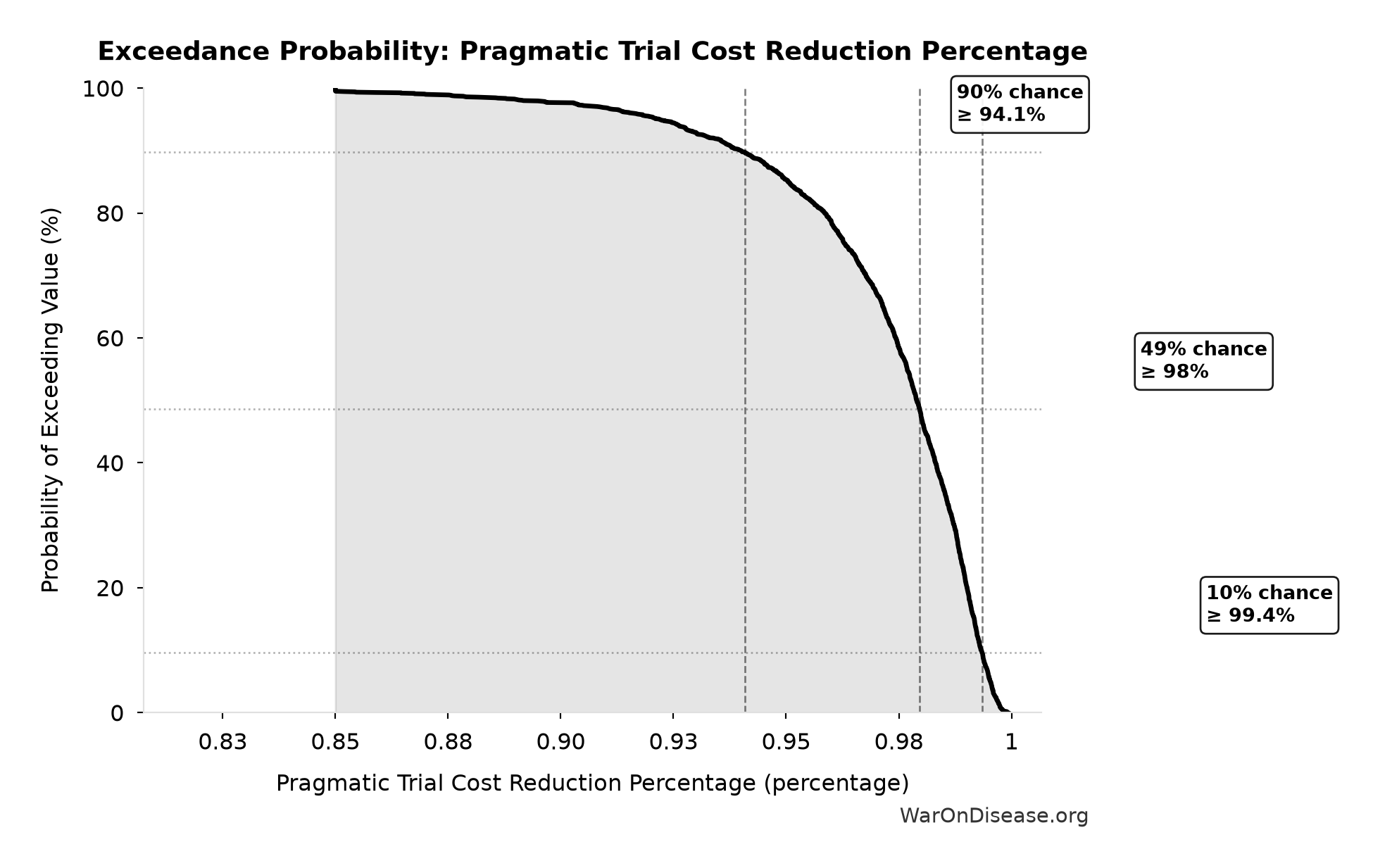
This exceedance probability chart shows the likelihood that Pragmatic Trial Cost Reduction Percentage will exceed any given threshold. The higher the curve at a threshold, the more likely the value exceeds it.
Reference Annual Trial Subsidies: $21.8 billion
Note📊 Details
Annual patient-level pragmatic trial subsidies after operating costs at the reference funding level
Inputs:
- Reference Annual Pragmatic Trial Funding: $21.8 billion
- Total Annual Pragmatic Trial Platform Operational Costs 🔢: $40 million
\[ \begin{gathered} Subsidies_{trial,ref} \\ = Funding_{trial,ref} - OPEX_{trial} \\ = \$21.8B - \$40M \\ = \$21.8B \end{gathered} \] where: \[ \begin{gathered} OPEX_{trial} \\ = Cost_{platform} + Cost_{staff} + Cost_{infra} \\ + Cost_{regulatory} + Cost_{community} \\ = \$15M + \$10M + \$8M + \$5M + \$2M \\ = \$40M \end{gathered} \] ✓ High confidence
Sensitivity Analysis
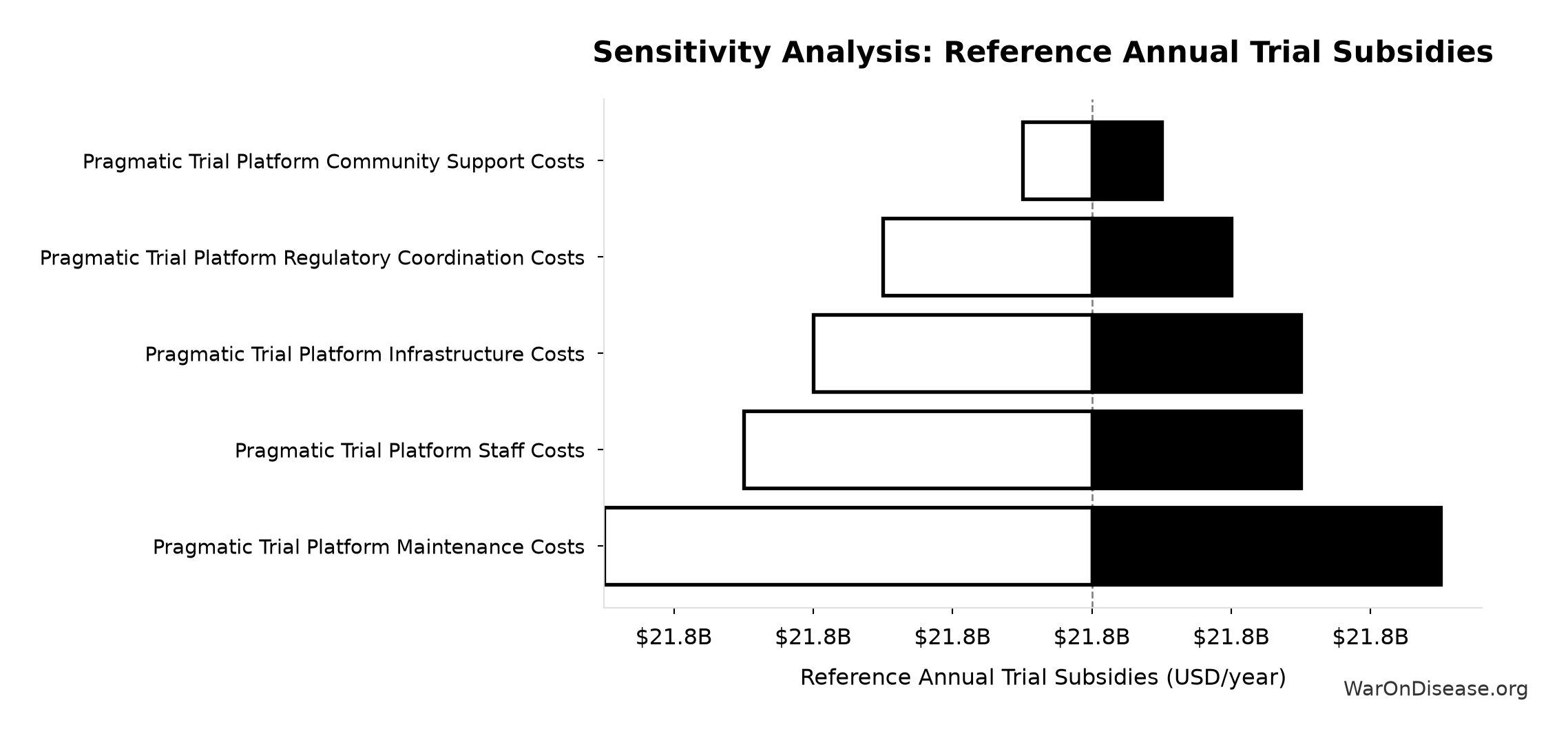
Sensitivity Indices for Reference Annual Trial Subsidies
Regression-based sensitivity showing which inputs explain the most variance in the output.
| Input Parameter | Sensitivity Coefficient | Interpretation |
|---|---|---|
| Total Annual Pragmatic Trial Platform Operational Costs (USD/year) | -1.0000 | Strong driver |
Interpretation: Standardized coefficients show the change in output (in SD units) per 1 SD change in input. Values near ±1 indicate strong influence; values exceeding ±1 may occur with correlated inputs.
Monte Carlo Distribution

Simulation Results Summary: Reference Annual Trial Subsidies
| Statistic | Value |
|---|---|
| Baseline (deterministic) | $21.8 billion |
| Mean (expected value) | $21.8 billion |
| Median (50th percentile) | $21.8 billion |
| Standard Deviation | $4.09 million |
| 90% Range (5th-95th percentile) | [$21.8 billion, $21.8 billion] |
The histogram shows 1,000 of the 10,000 Monte Carlo draws for Reference Annual Trial Subsidies; the summary statistics use all 10,000. The exceedance curve (right) shows the probability of the outcome exceeding any given value.
Exceedance Probability
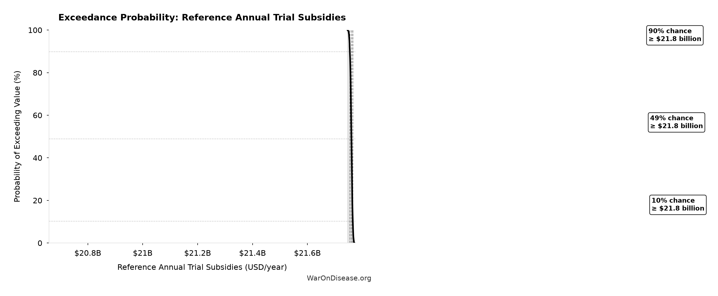
This exceedance probability chart shows the likelihood that Reference Annual Trial Subsidies will exceed any given threshold. The higher the curve at a threshold, the more likely the value exceeds it.
Diseases Without Effective Treatment: 6,650 diseases
Note📊 Details
Number of diseases without effective treatment. 95% of 7,000 rare diseases lack FDA-approved treatment (per Orphanet 2024). This represents the therapeutic search space that remains unexplored.
Inputs:
- Total Number of Rare Diseases Globally 📊: 7,000 diseases (95% CI: 6,000 diseases - 10,000 diseases)
\[ \begin{gathered} N_{untreated} \\ = N_{rare} \times 0.95 \\ = 7{,}000 \times 0.95 \\ = 6{,}650 \end{gathered} \]
Methodology:36
~ Medium confidence
Sensitivity Analysis
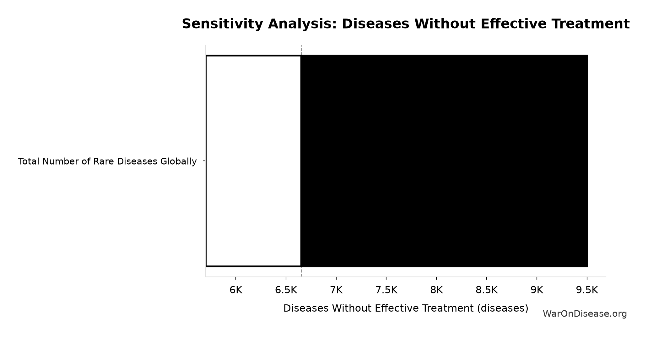
Sensitivity Indices for Diseases Without Effective Treatment
Regression-based sensitivity showing which inputs explain the most variance in the output.
| Input Parameter | Sensitivity Coefficient | Interpretation |
|---|---|---|
| Total Number of Rare Diseases Globally (diseases) | 1.0000 | Strong driver |
Interpretation: Standardized coefficients show the change in output (in SD units) per 1 SD change in input. Values near ±1 indicate strong influence; values exceeding ±1 may occur with correlated inputs.
Monte Carlo Distribution
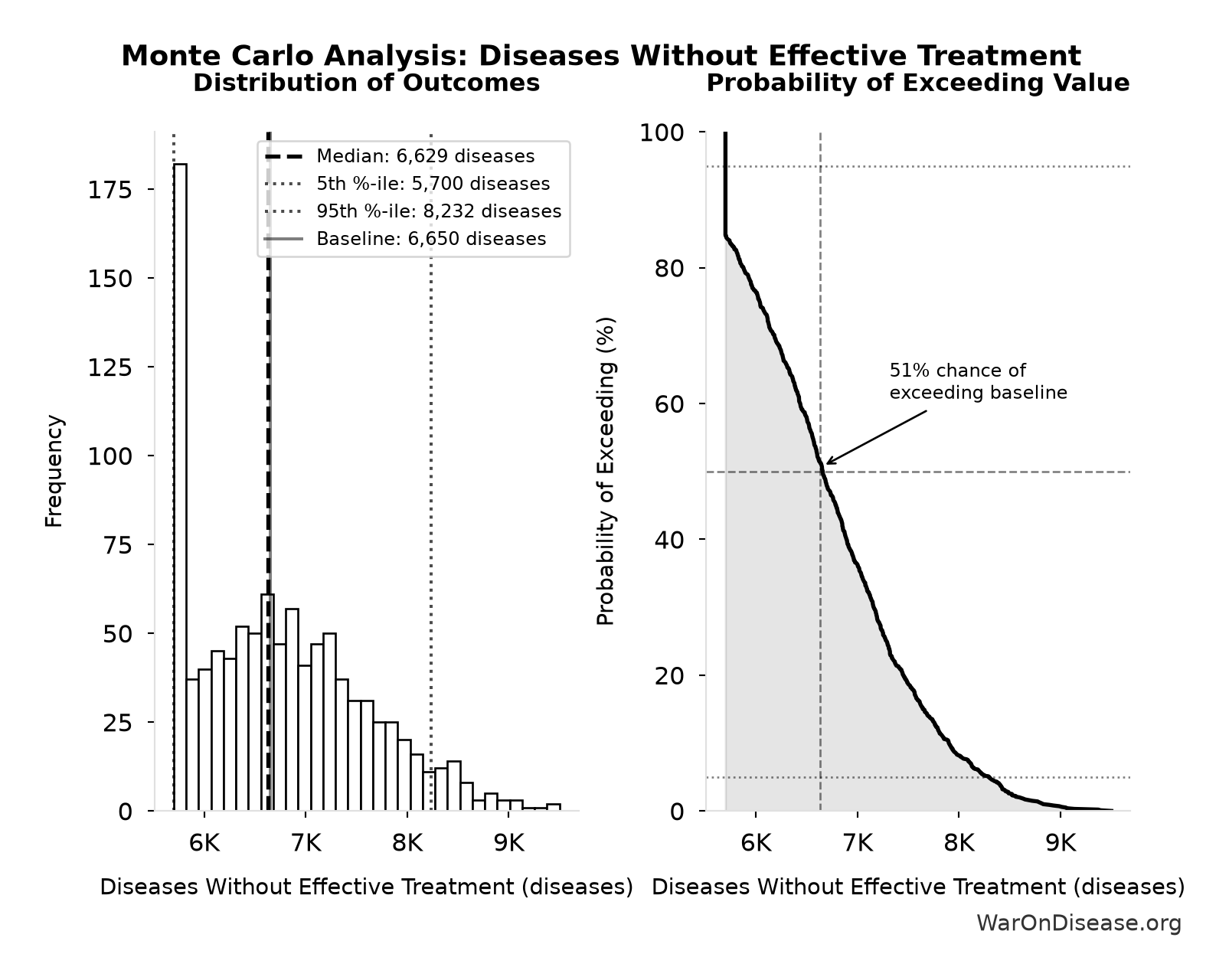
Simulation Results Summary: Diseases Without Effective Treatment
| Statistic | Value |
|---|---|
| Baseline (deterministic) | 6,650 |
| Mean (expected value) | 6,718 |
| Median (50th percentile) | 6,629 |
| Standard Deviation | 827 |
| 90% Range (5th-95th percentile) | [5,700, 8,232] |
The histogram shows 1,000 of the 10,000 Monte Carlo draws for Diseases Without Effective Treatment; the summary statistics use all 10,000. The exceedance curve (right) shows the probability of the outcome exceeding any given value.
Exceedance Probability
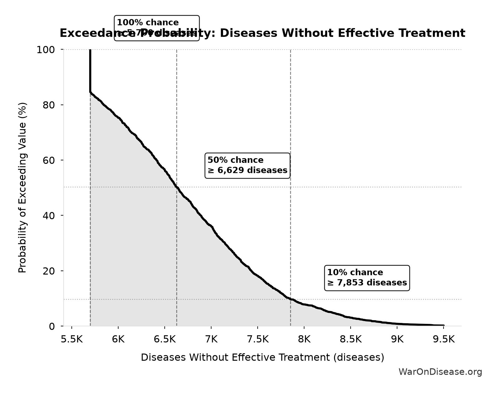
This exceedance probability chart shows the likelihood that Diseases Without Effective Treatment will exceed any given threshold. The higher the curve at a threshold, the more likely the value exceeds it.
Total Drugs Approved Since 1962: 3,100 drugs
Note📊 Details
Estimated total drugs approved globally since 1962 (62 years × average approval rate). Conservative: uses current rate, actual historical rate was lower in 1960s-80s.
Inputs:
- Average Annual New Drug Approvals Globally 📊: 50 drugs/year (95% CI: 45 drugs/year - 60 drugs/year)
\[ \begin{gathered} N_{drugs,62} \\ = Drugs_{ann,curr} \times 62 \\ = 50 \times 62 \\ = 3{,}100 \end{gathered} \]
Methodology:8
~ Medium confidence
Sensitivity Analysis
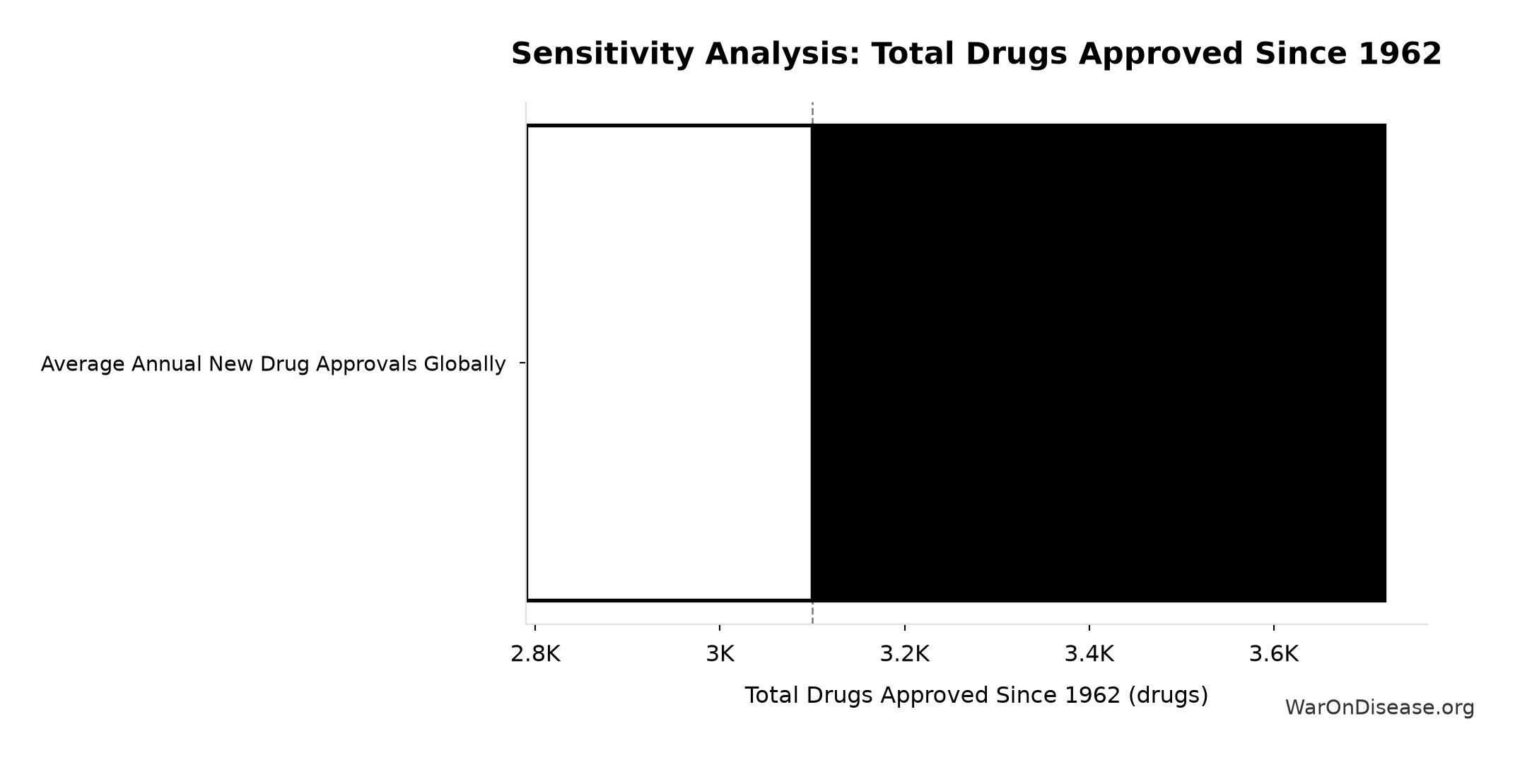
Sensitivity Indices for Total Drugs Approved Since 1962
Regression-based sensitivity showing which inputs explain the most variance in the output.
| Input Parameter | Sensitivity Coefficient | Interpretation |
|---|---|---|
| Average Annual New Drug Approvals Globally (drugs/year) | 1.0000 | Strong driver |
Interpretation: Standardized coefficients show the change in output (in SD units) per 1 SD change in input. Values near ±1 indicate strong influence; values exceeding ±1 may occur with correlated inputs.
Monte Carlo Distribution
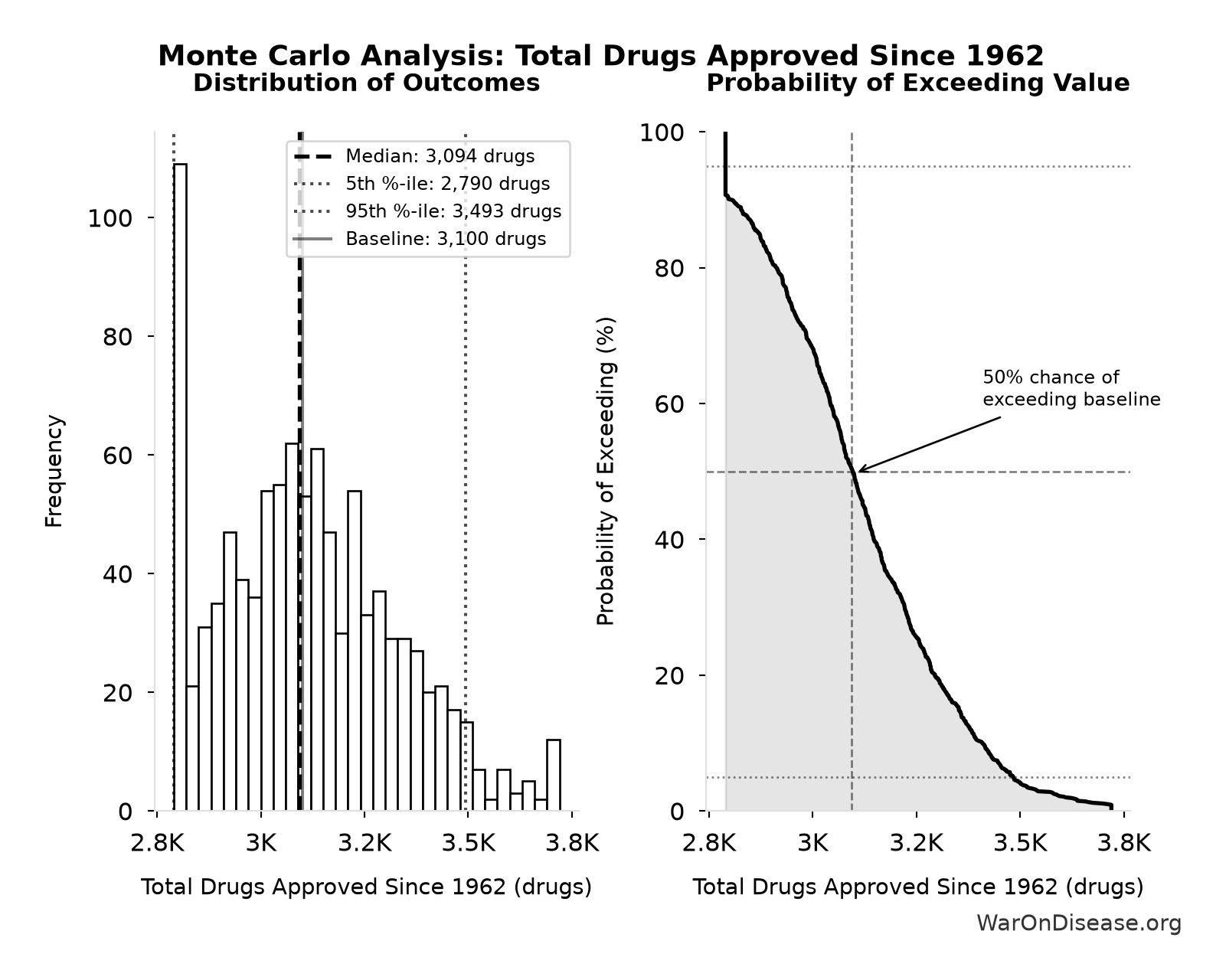
Simulation Results Summary: Total Drugs Approved Since 1962
| Statistic | Value |
|---|---|
| Baseline (deterministic) | 3,100 |
| Mean (expected value) | 3,109 |
| Median (50th percentile) | 3,094 |
| Standard Deviation | 217 |
| 90% Range (5th-95th percentile) | [2,790, 3,493] |
The histogram shows 1,000 of the 10,000 Monte Carlo draws for Total Drugs Approved Since 1962; the summary statistics use all 10,000. The exceedance curve (right) shows the probability of the outcome exceeding any given value.
Exceedance Probability
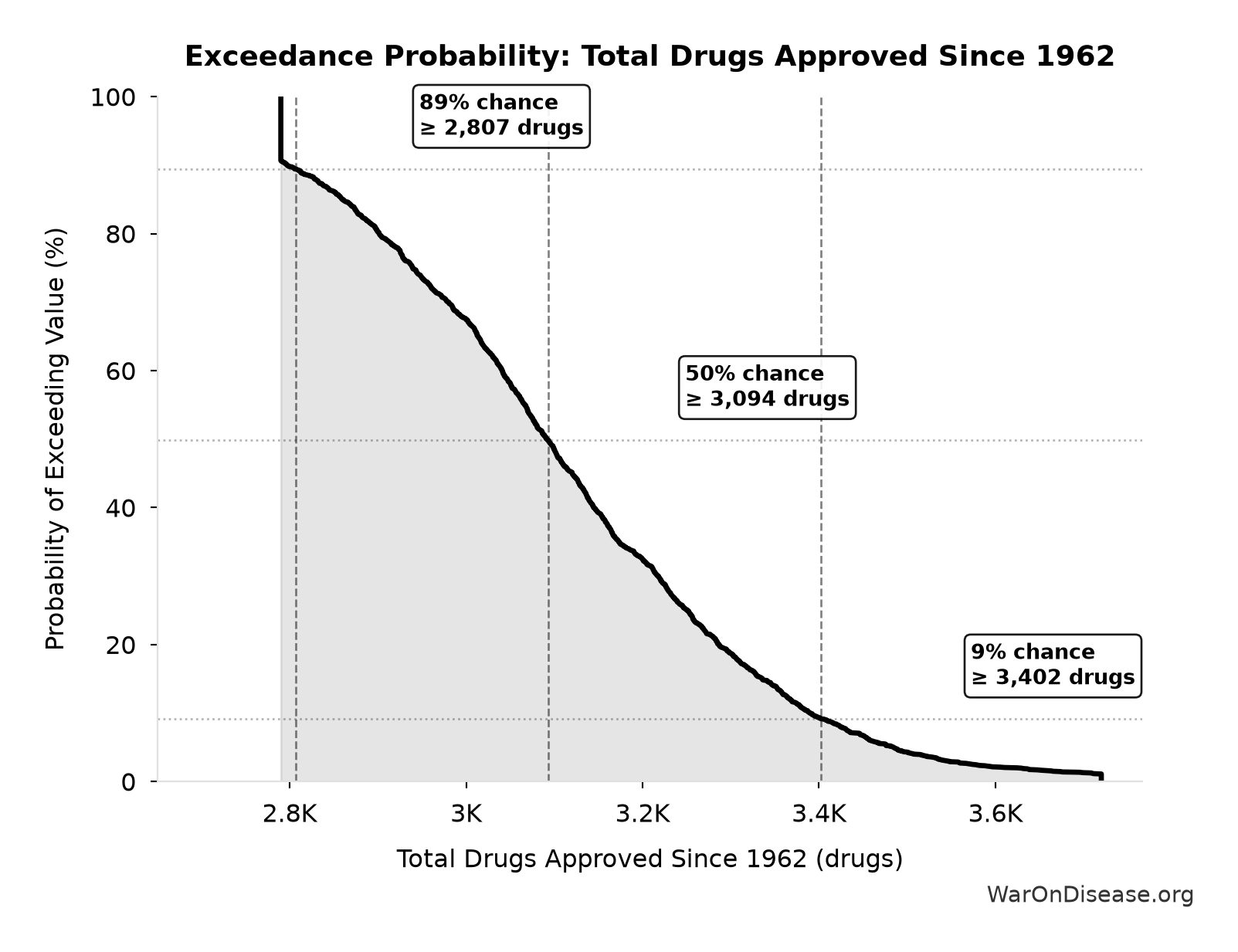
This exceedance probability chart shows the likelihood that Total Drugs Approved Since 1962 will exceed any given threshold. The higher the curve at a threshold, the more likely the value exceeds it.
Drug Cost Increase: 1980s to Current: 13.4x
Note📊 Details
Drug development cost increase from 1980s to current
Inputs:
- Drug Development Cost (1980s) 📊: $194 million (95% CI: $146 million - $242 million)
- Pharma Drug Development Cost (Current System) 📊: $2.6 billion (95% CI: $1.5 billion - $4 billion)
\[ \begin{gathered} k_{cost,80s} \\ = \frac{Cost_{dev,curr}}{Cost_{dev,80s}} \\ = \frac{\$2.6B}{\$194M} \\ = 13.4 \end{gathered} \]
Methodology:37
✓ High confidence
Sensitivity Analysis
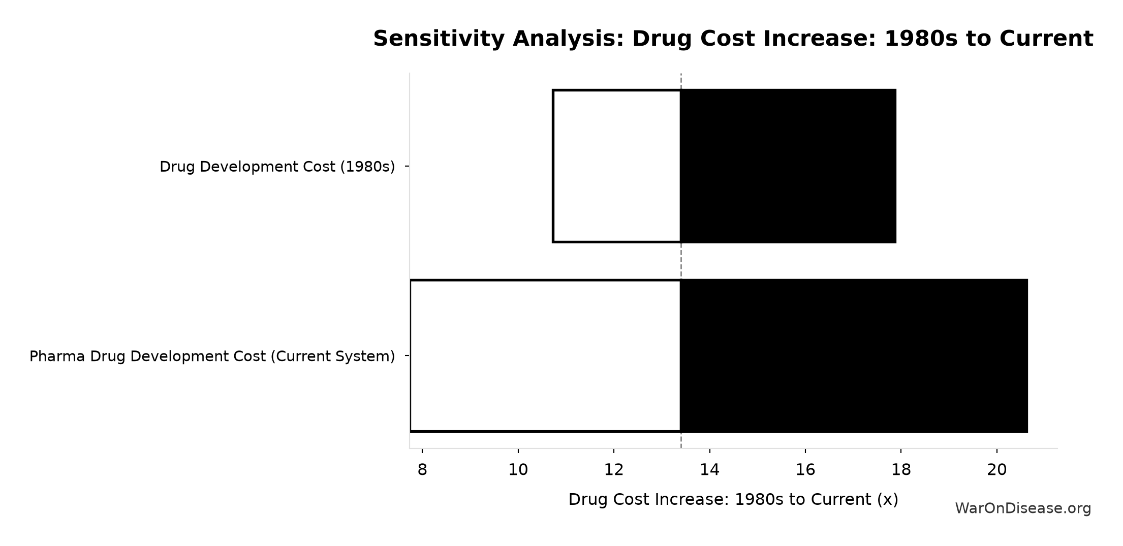
Sensitivity Indices for Drug Cost Increase: 1980s to Current
Regression-based sensitivity showing which inputs explain the most variance in the output.
| Input Parameter | Sensitivity Coefficient | Interpretation |
|---|---|---|
| Pharma Drug Development Cost (Current System) (USD) | 0.8327 | Strong driver |
| Drug Development Cost (1980s) (USD) | -0.5396 | Strong driver |
Interpretation: Standardized coefficients show the change in output (in SD units) per 1 SD change in input. Values near ±1 indicate strong influence; values exceeding ±1 may occur with correlated inputs.
Monte Carlo Distribution
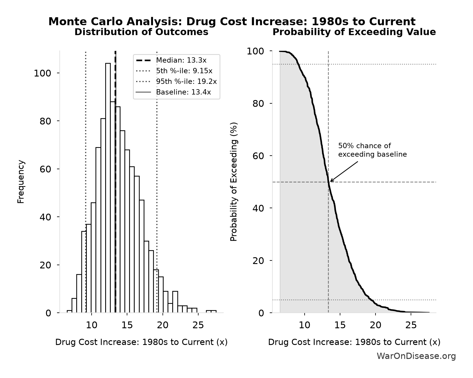
Simulation Results Summary: Drug Cost Increase: 1980s to Current
| Statistic | Value |
|---|---|
| Baseline (deterministic) | 13.4x |
| Mean (expected value) | 13.6x |
| Median (50th percentile) | 13.3x |
| Standard Deviation | 3.06x |
| 90% Range (5th-95th percentile) | [9.15x, 19.2x] |
The histogram shows 1,000 of the 10,000 Monte Carlo draws for Drug Cost Increase: 1980s to Current; the summary statistics use all 10,000. The exceedance curve (right) shows the probability of the outcome exceeding any given value.
Exceedance Probability
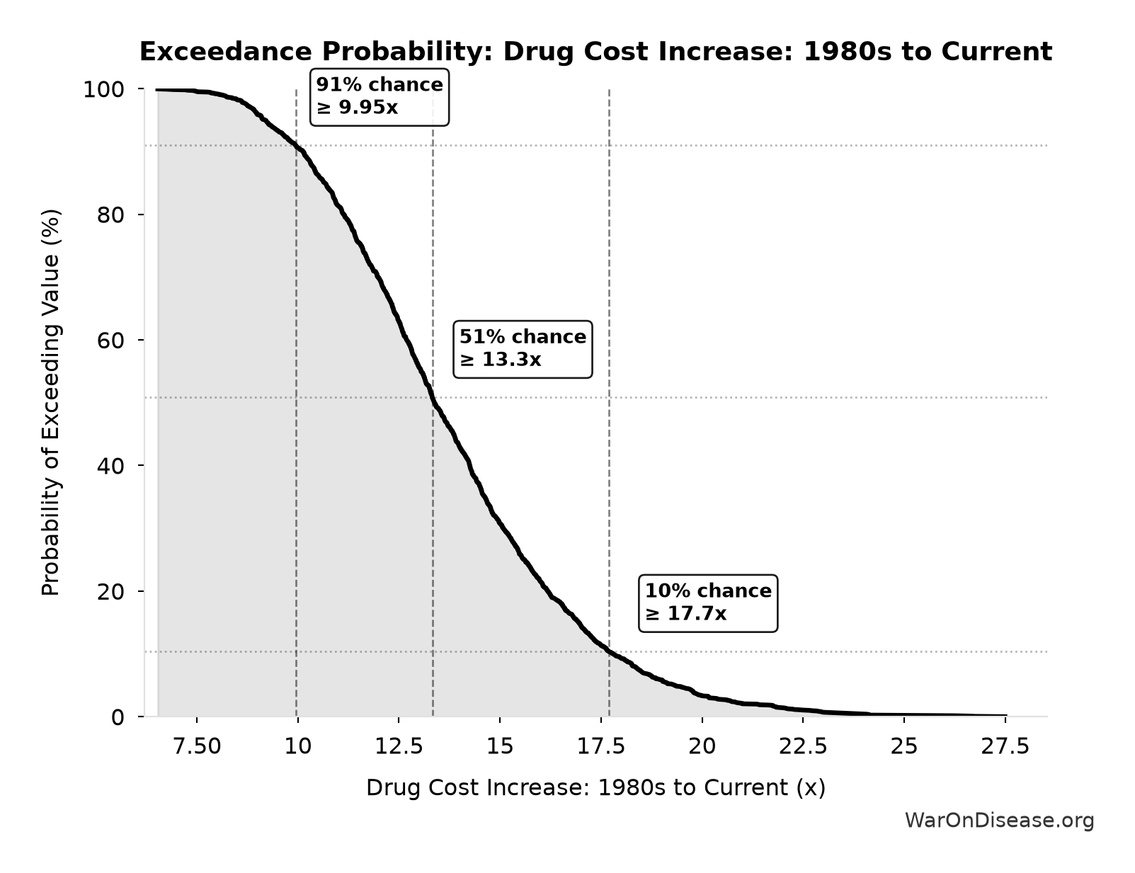
This exceedance probability chart shows the likelihood that Drug Cost Increase: 1980s to Current will exceed any given threshold. The higher the curve at a threshold, the more likely the value exceeds it.
Drug Cost Increase: Pre-1962 to Current: 105x
Note📊 Details
Drug development cost increase from pre-1962 to current
Inputs:
- Pharma Drug Development Cost (Current System) 📊: $2.6 billion (95% CI: $1.5 billion - $4 billion)
- Pre-1962 Drug Development Cost (2024 Dollars) 📊: $24.7 million (95% CI: $19.5 million - $30 million)
\[ \begin{gathered} k_{cost,pre62} \\ = \frac{Cost_{dev,curr}}{Cost_{pre62,24}} \\ = \frac{\$2.6B}{\$24.7M} \\ = 105 \end{gathered} \]
Methodology:27
✓ High confidence
Sensitivity Analysis
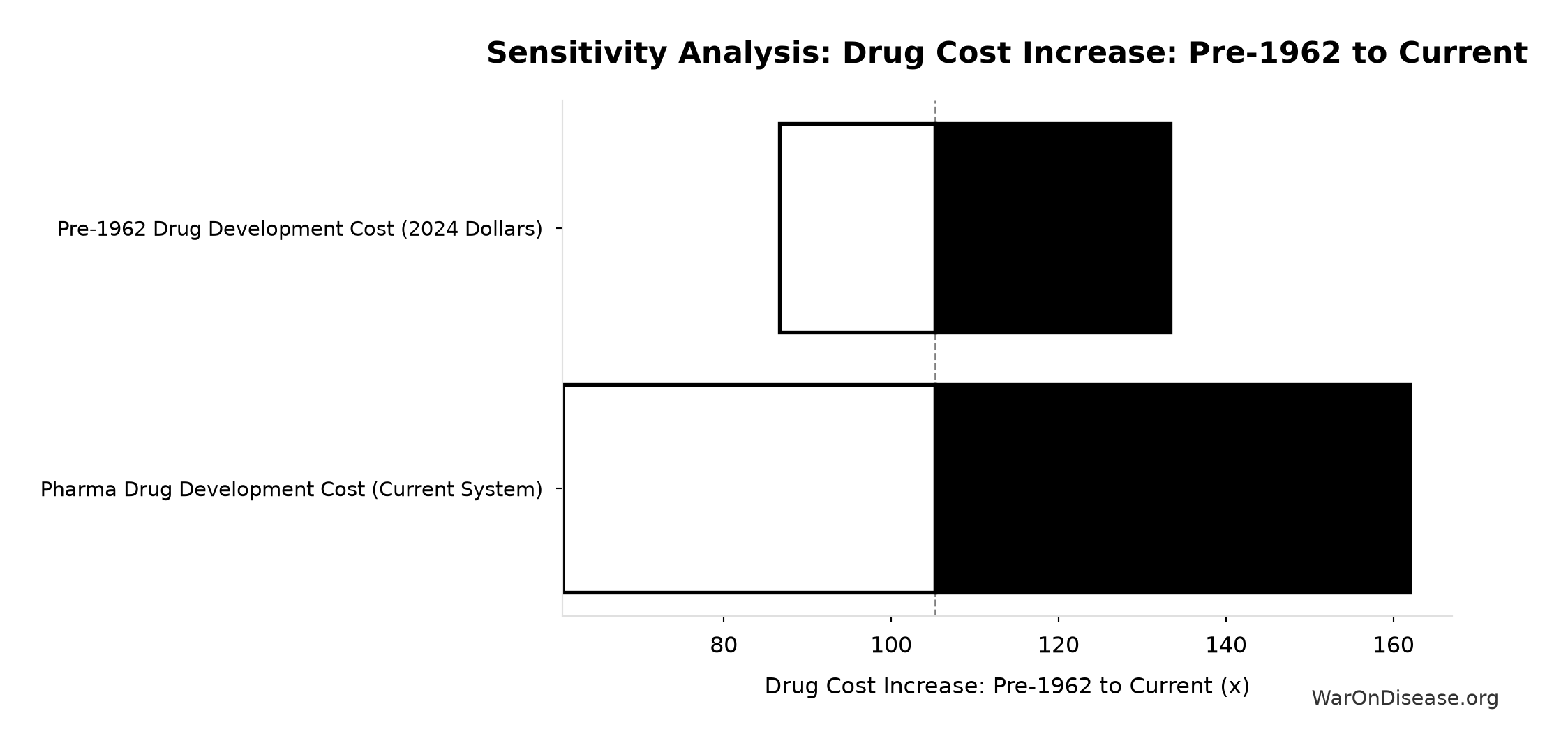
Sensitivity Indices for Drug Cost Increase: Pre-1962 to Current
Regression-based sensitivity showing which inputs explain the most variance in the output.
| Input Parameter | Sensitivity Coefficient | Interpretation |
|---|---|---|
| Pharma Drug Development Cost (Current System) (USD) | 0.8709 | Strong driver |
| Pre-1962 Drug Development Cost (2024 Dollars) (USD) | -0.4736 | Moderate driver |
Interpretation: Standardized coefficients show the change in output (in SD units) per 1 SD change in input. Values near ±1 indicate strong influence; values exceeding ±1 may occur with correlated inputs.
Monte Carlo Distribution
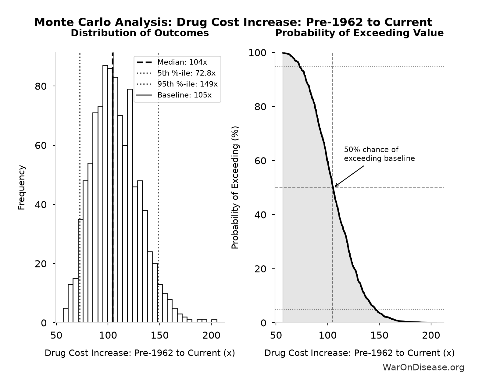
Simulation Results Summary: Drug Cost Increase: Pre-1962 to Current
| Statistic | Value |
|---|---|
| Baseline (deterministic) | 105x |
| Mean (expected value) | 107x |
| Median (50th percentile) | 104x |
| Standard Deviation | 22.9x |
| 90% Range (5th-95th percentile) | [72.8x, 149x] |
The histogram shows 1,000 of the 10,000 Monte Carlo draws for Drug Cost Increase: Pre-1962 to Current; the summary statistics use all 10,000. The exceedance curve (right) shows the probability of the outcome exceeding any given value.
Exceedance Probability
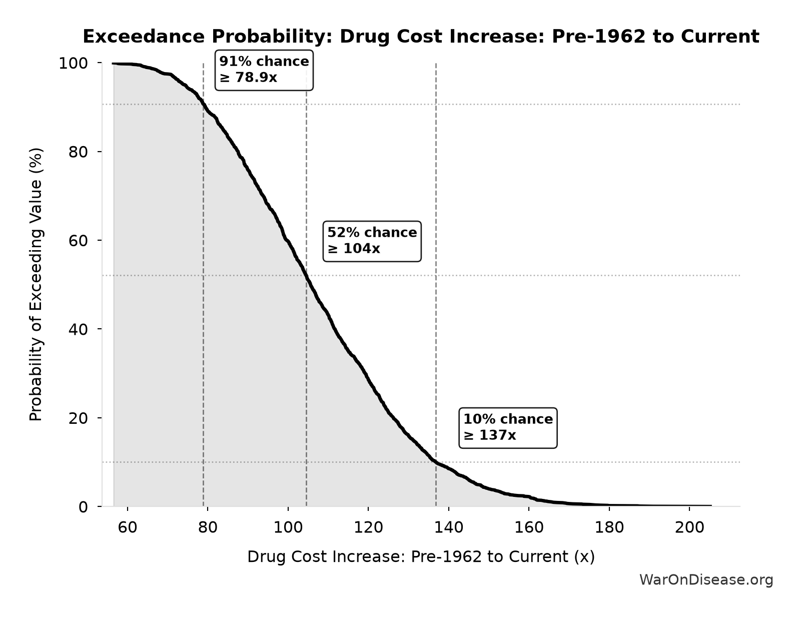
This exceedance probability chart shows the likelihood that Drug Cost Increase: Pre-1962 to Current will exceed any given threshold. The higher the curve at a threshold, the more likely the value exceeds it.
Possible Drug-Disease Combinations: 9.5 million combinations
Note📊 Details
Total possible drug-disease combinations using existing safe compounds
Inputs:
- Safe Compounds Available for Testing: 9,500 compounds (95% CI: 7,000 compounds - 12,000 compounds)
- Trial-Relevant Diseases: 1,000 diseases (95% CI: 800 diseases - 1,200 diseases)
\[ \begin{gathered} N_{combos} \\ = N_{safe} \times N_{diseases,trial} \\ = 9{,}500 \times 1{,}000 \\ = 9.5M \end{gathered} \]
✓ High confidence
Sensitivity Analysis
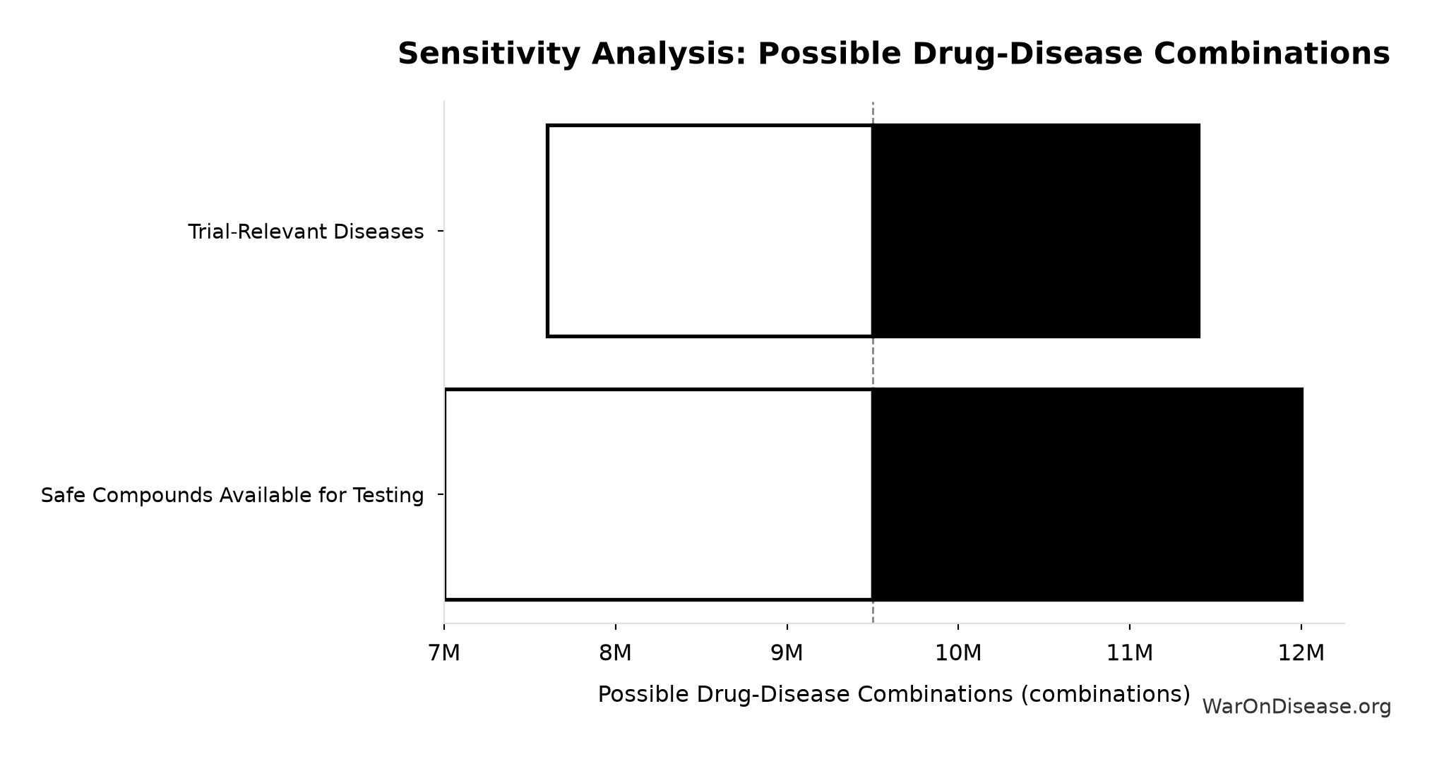
Sensitivity Indices for Possible Drug-Disease Combinations
Regression-based sensitivity showing which inputs explain the most variance in the output.
| Input Parameter | Sensitivity Coefficient | Interpretation |
|---|---|---|
| Safe Compounds Available for Testing (compounds) | 0.7847 | Strong driver |
| Trial-Relevant Diseases (diseases) | 0.5990 | Strong driver |
Interpretation: Standardized coefficients show the change in output (in SD units) per 1 SD change in input. Values near ±1 indicate strong influence; values exceeding ±1 may occur with correlated inputs.
Monte Carlo Distribution
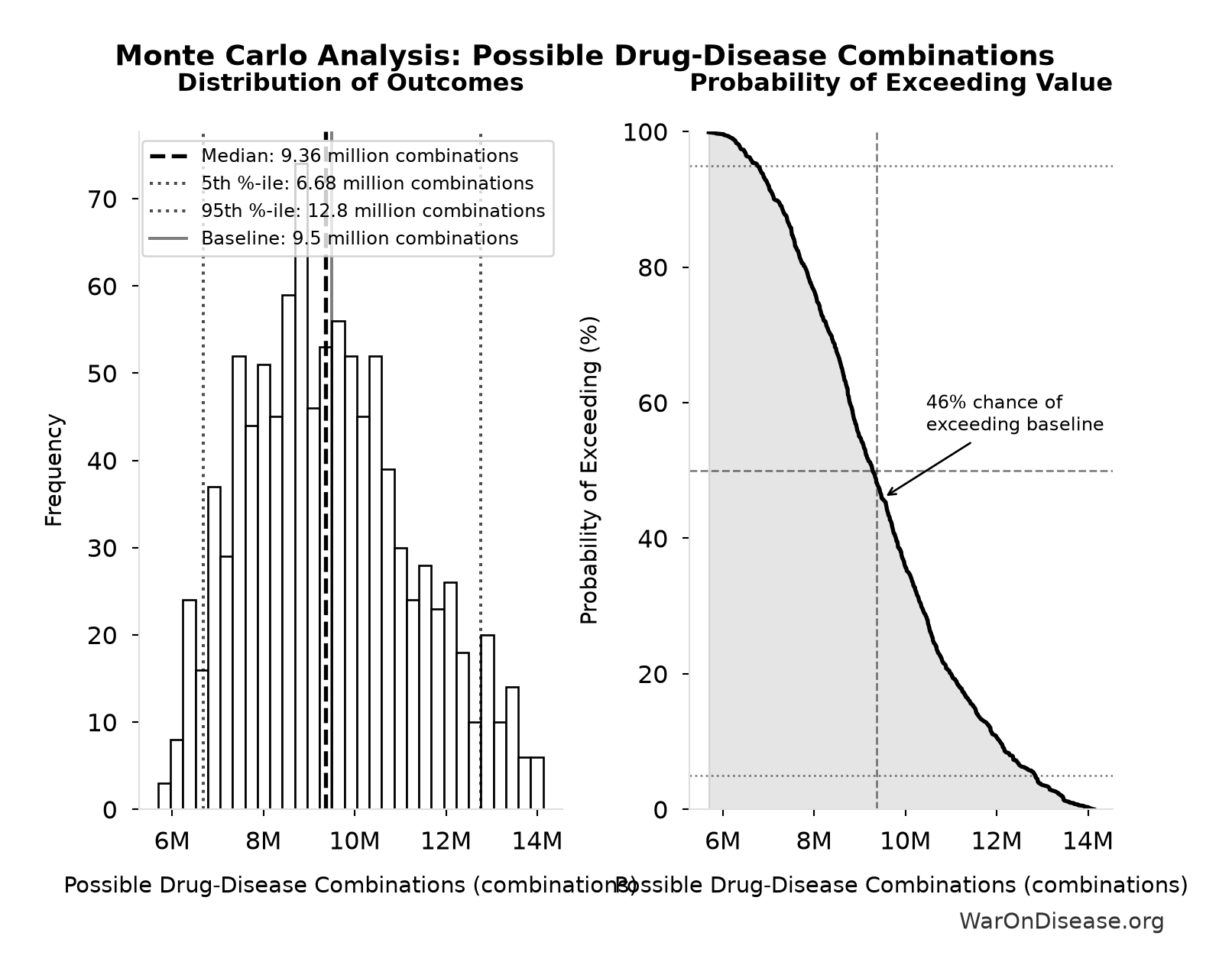
Simulation Results Summary: Possible Drug-Disease Combinations
| Statistic | Value |
|---|---|
| Baseline (deterministic) | 9.5 million |
| Mean (expected value) | 9.48 million |
| Median (50th percentile) | 9.36 million |
| Standard Deviation | 1.83 million |
| 90% Range (5th-95th percentile) | [6.68 million, 12.8 million] |
The histogram shows 1,000 of the 10,000 Monte Carlo draws for Possible Drug-Disease Combinations; the summary statistics use all 10,000. The exceedance curve (right) shows the probability of the outcome exceeding any given value.
Exceedance Probability
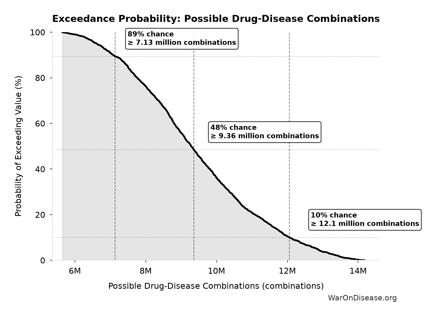
This exceedance probability chart shows the likelihood that Possible Drug-Disease Combinations will exceed any given threshold. The higher the curve at a threshold, the more likely the value exceeds it.
Cumulative Efficacy Testing Cost (1962-2024): $4.84 trillion
Note📊 Details
Cumulative Phase 2/3 efficacy testing cost since 1962. Uses direct Phase 2/3 cost per drug - this is a LOWER BOUND because it excludes opportunity cost of delays, compounds abandoned due to cost barrier, and regulatory overhead.
Inputs:
- Pharma Phase 2/3 Cost Barrier Per Drug: $1.56 billion (SE: ±$200 million)
- Total Drugs Approved Since 1962 🔢: 3,100 drugs
\[ \begin{gathered} Cost_{eff,cumul} \\ = Cost_{P2+P3} \times N_{drugs,62} \\ = \$1.56B \times 3{,}100 \\ = \$4.84T \end{gathered} \] where: \[ \begin{gathered} N_{drugs,62} \\ = Drugs_{ann,curr} \times 62 \\ = 50 \times 62 \\ = 3{,}100 \end{gathered} \] ~ Medium confidence
Sensitivity Analysis
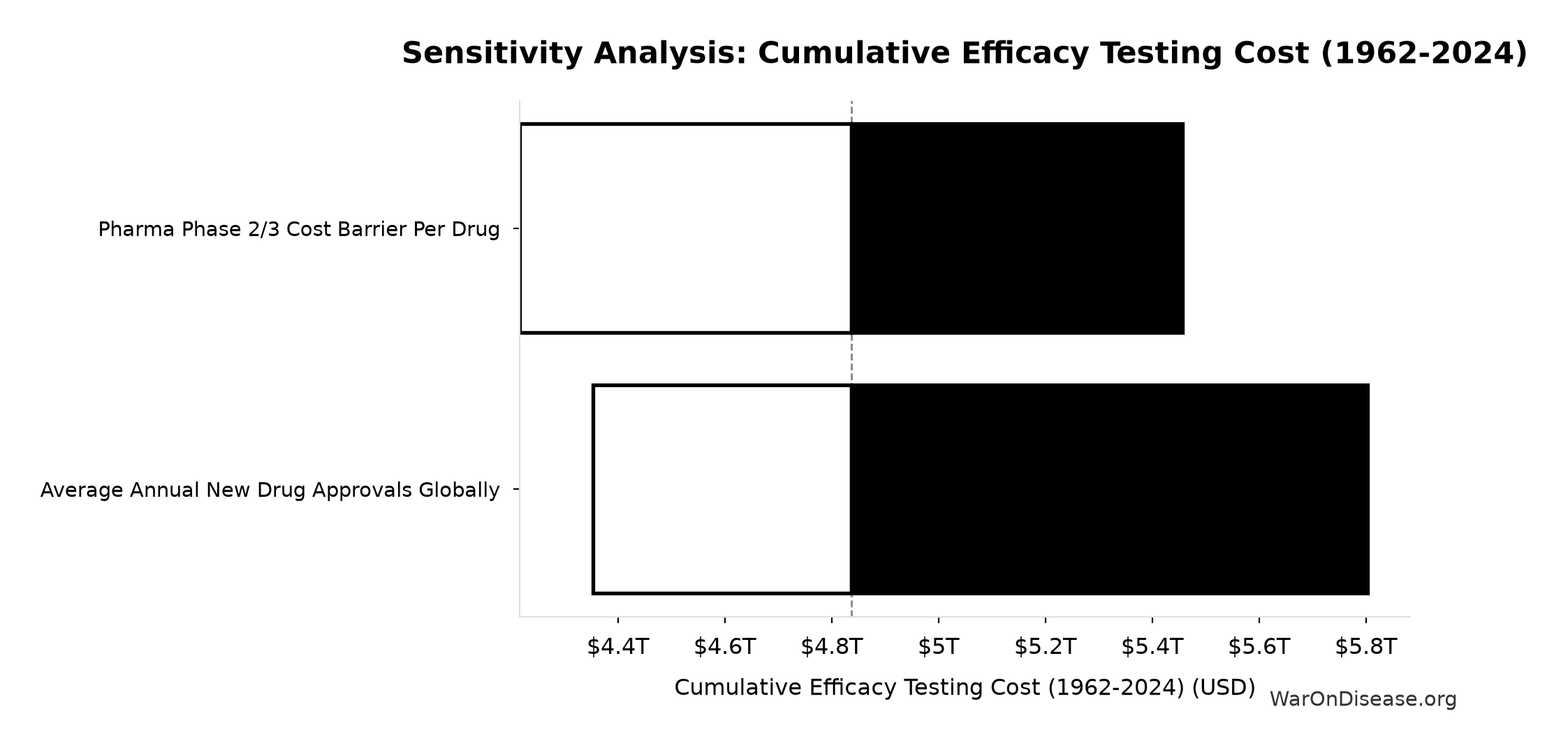
Sensitivity Indices for Cumulative Efficacy Testing Cost (1962-2024)
Regression-based sensitivity showing which inputs explain the most variance in the output.
| Input Parameter | Sensitivity Coefficient | Interpretation |
|---|---|---|
| Pharma Phase 2/3 Cost Barrier Per Drug (USD) | 0.8781 | Strong driver |
| Total Drugs Approved Since 1962 (drugs) | 0.4846 | Moderate driver |
Interpretation: Standardized coefficients show the change in output (in SD units) per 1 SD change in input. Values near ±1 indicate strong influence; values exceeding ±1 may occur with correlated inputs.
Monte Carlo Distribution
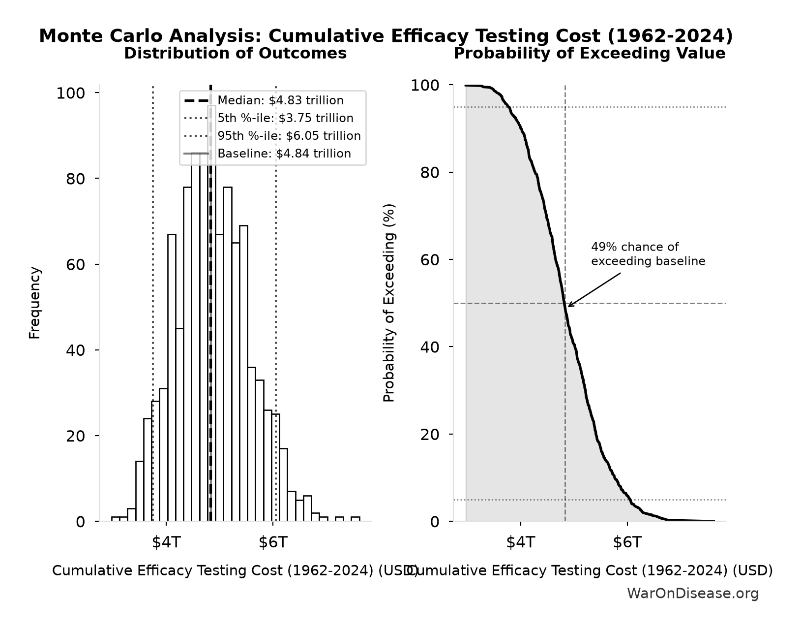
Simulation Results Summary: Cumulative Efficacy Testing Cost (1962-2024)
| Statistic | Value |
|---|---|
| Baseline (deterministic) | $4.84 trillion |
| Mean (expected value) | $4.86 trillion |
| Median (50th percentile) | $4.83 trillion |
| Standard Deviation | $701 billion |
| 90% Range (5th-95th percentile) | [$3.75 trillion, $6.05 trillion] |
The histogram shows 1,000 of the 10,000 Monte Carlo draws for Cumulative Efficacy Testing Cost (1962-2024); the summary statistics use all 10,000. The exceedance curve (right) shows the probability of the outcome exceeding any given value.
Exceedance Probability
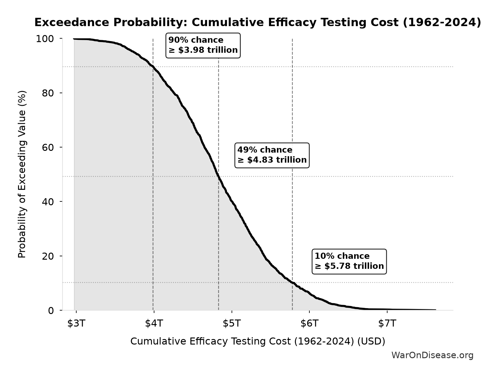
This exceedance probability chart shows the likelihood that Cumulative Efficacy Testing Cost (1962-2024) will exceed any given threshold. The higher the curve at a threshold, the more likely the value exceeds it.
Efficacy Lag Deaths (9/11 Equivalents): 34,132 9/11s
Note📊 Details
Total deaths from efficacy lag expressed in 9/11 equivalents. Makes the mortality cost viscerally understandable: how many September 11ths worth of deaths did the 1962 efficacy requirements cause?
Inputs:
- Total Deaths from Historical Progress Delays 🔢: 102 million deaths
- September 11 Deaths 📊: 2,977 people
\[ \begin{gathered} N_{9/11,equiv} \\ = \frac{Deaths_{lag,total}}{N_{9/11}} \\ = \frac{102M}{2{,}980} \\ = 34{,}100 \end{gathered} \] where: \[ \begin{gathered} Deaths_{lag,total} \\ = Lives_{saved,annual} \times T_{lag} \\ = 12.4M \times 8.2 \\ = 102M \end{gathered} \] where: \[ \begin{gathered} Lives_{saved,annual} \\ = \frac{LY_{saved,annual}}{T_{ext}} \\ = \frac{149M}{12} \\ = 12.4M \end{gathered} \] ~ Medium confidence
Sensitivity Analysis
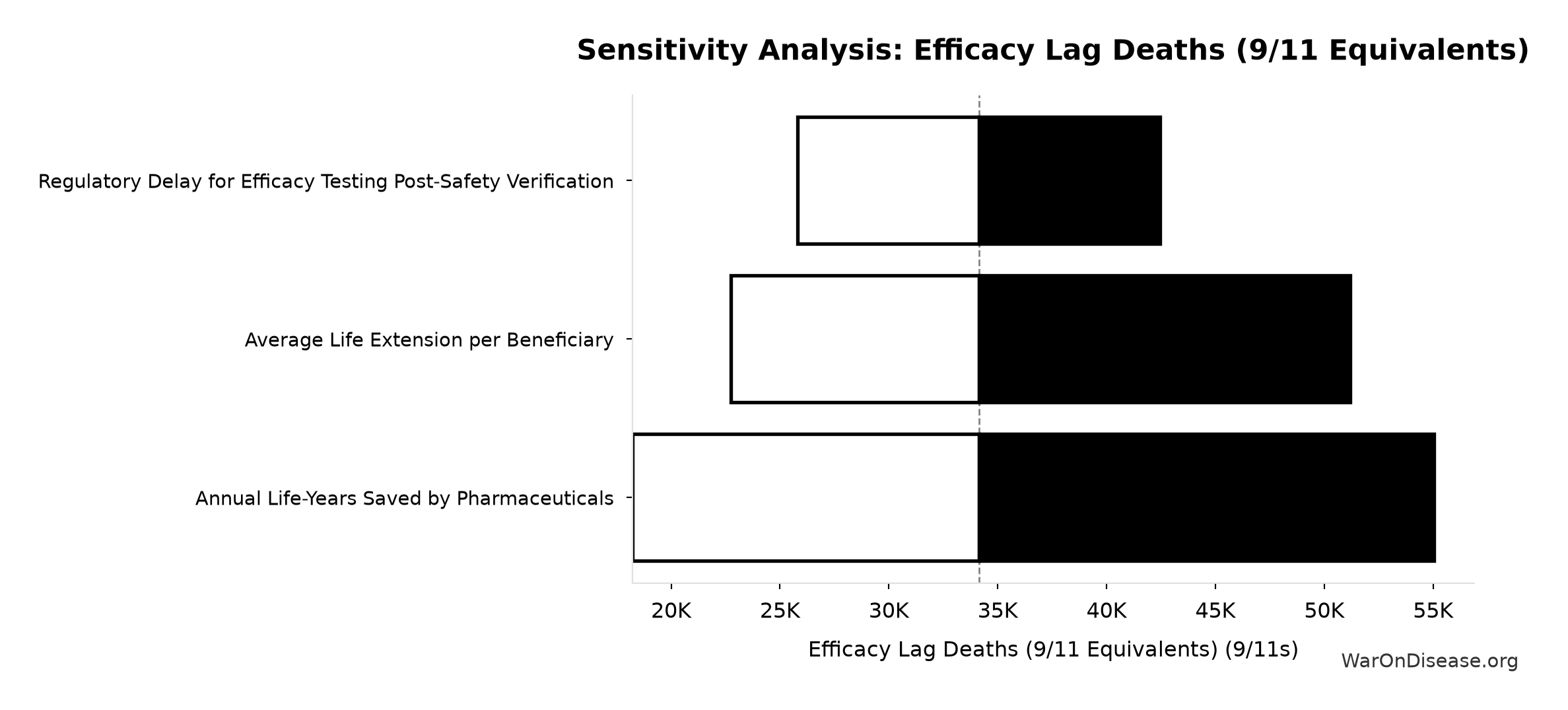
Sensitivity Indices for Efficacy Lag Deaths (9/11 Equivalents)
Regression-based sensitivity showing which inputs explain the most variance in the output.
| Input Parameter | Sensitivity Coefficient | Interpretation |
|---|---|---|
| Total Deaths from Historical Progress Delays (deaths) | 1.0000 | Strong driver |
Interpretation: Standardized coefficients show the change in output (in SD units) per 1 SD change in input. Values near ±1 indicate strong influence; values exceeding ±1 may occur with correlated inputs.
Monte Carlo Distribution
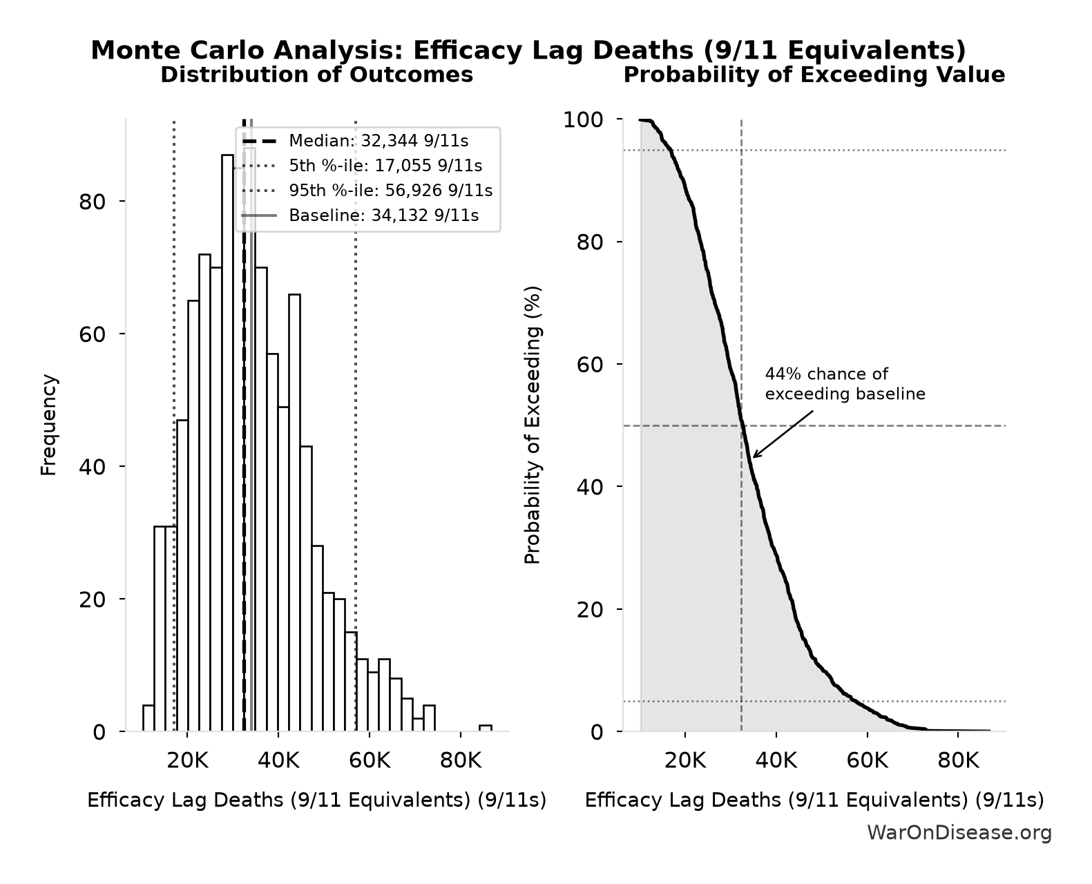
Simulation Results Summary: Efficacy Lag Deaths (9/11 Equivalents)
| Statistic | Value |
|---|---|
| Baseline (deterministic) | 34,132 |
| Mean (expected value) | 34,033 |
| Median (50th percentile) | 32,344 |
| Standard Deviation | 12,202 |
| 90% Range (5th-95th percentile) | [17,055, 56,926] |
The histogram shows 1,000 of the 10,000 Monte Carlo draws for Efficacy Lag Deaths (9/11 Equivalents); the summary statistics use all 10,000. The exceedance curve (right) shows the probability of the outcome exceeding any given value.
Exceedance Probability
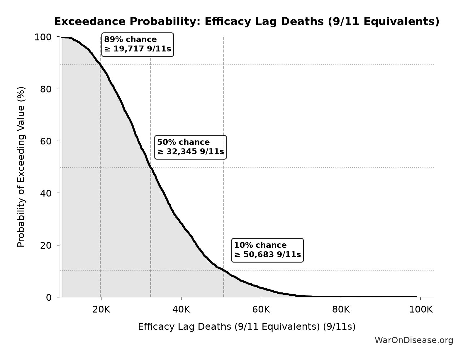
This exceedance probability chart shows the likelihood that Efficacy Lag Deaths (9/11 Equivalents) will exceed any given threshold. The higher the curve at a threshold, the more likely the value exceeds it.
Treatment Delay YLD - Annual: 2.01 billion DALYs
Note📊 Details
Annual YLD from treatment delay: patients receiving chronic disease treatment would have collectively avoided this disability if treatments were available 8.2 years earlier. Represents morbidity burden for treatment beneficiaries (distinct from mortality burden).
Inputs:
- Annual Chronic Disease Patients Treated 🔢: 982 million people
- Regulatory Delay for Efficacy Testing Post-Safety Verification 📊: 8.2 years (SE: ±2 years)
- Treatment Disability Reduction 📊: 0.25 weight (95% CI: 0.15 weight - 0.35 weight)
\[ \begin{gathered} YLD_{treat\_delay} \\ = N_{treated} \times T_{lag} \times \Delta DW_{treat} \\ = 982M \times 8.2 \times 0.25 \\ = 2.01B \end{gathered} \] where: \[ \begin{gathered} N_{treated} \\ = DOT_{chronic} \times 0.000767 \\ = 1.28T \times 0.000767 \\ = 982M \end{gathered} \] ? Low confidence
Sensitivity Analysis
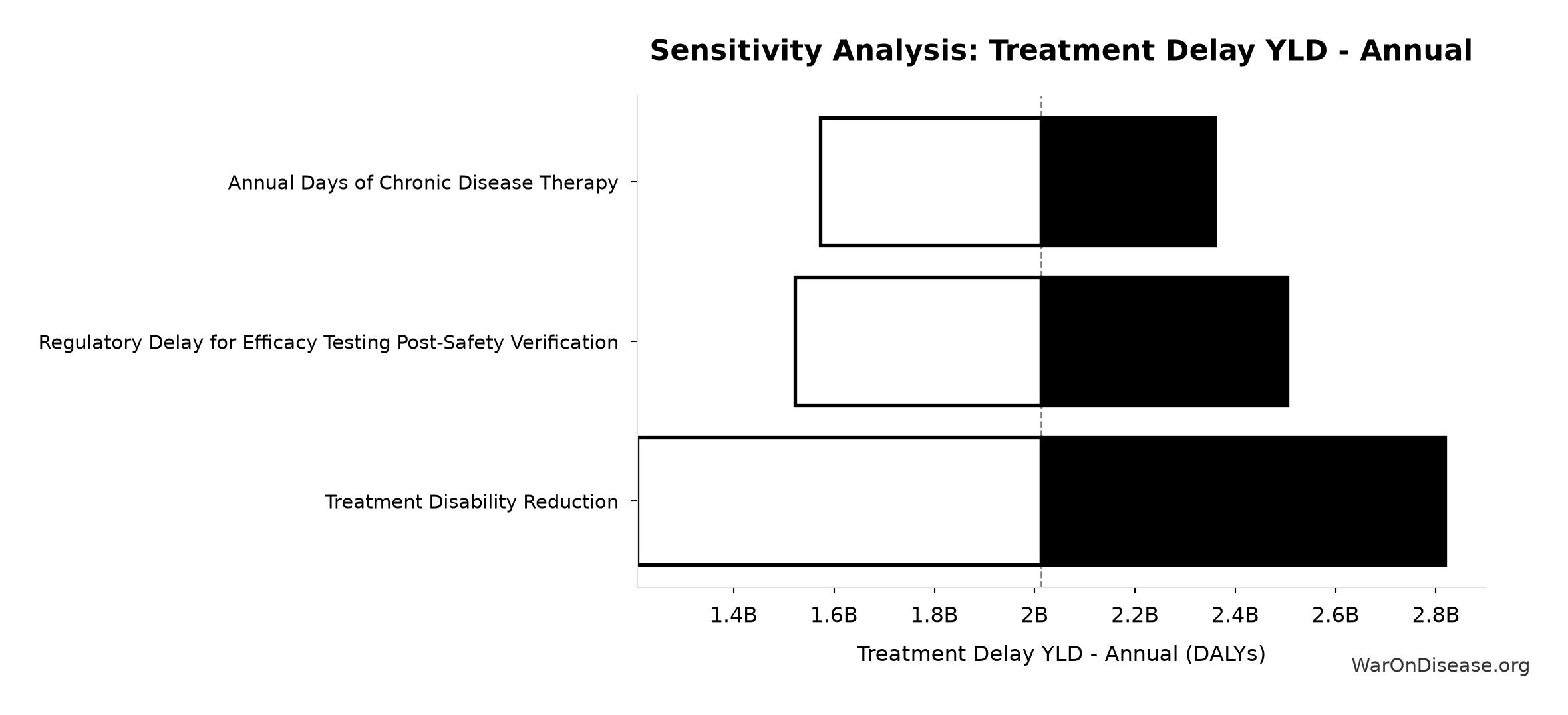
Sensitivity Indices for Treatment Delay YLD - Annual
Regression-based sensitivity showing which inputs explain the most variance in the output.
| Input Parameter | Sensitivity Coefficient | Interpretation |
|---|---|---|
| Regulatory Delay for Efficacy Testing Post-Safety Verification (years) | 0.7122 | Strong driver |
| Treatment Disability Reduction (weight) | 0.5988 | Strong driver |
| Annual Chronic Disease Patients Treated (people) | 0.2936 | Weak driver |
Interpretation: Standardized coefficients show the change in output (in SD units) per 1 SD change in input. Values near ±1 indicate strong influence; values exceeding ±1 may occur with correlated inputs.
Monte Carlo Distribution
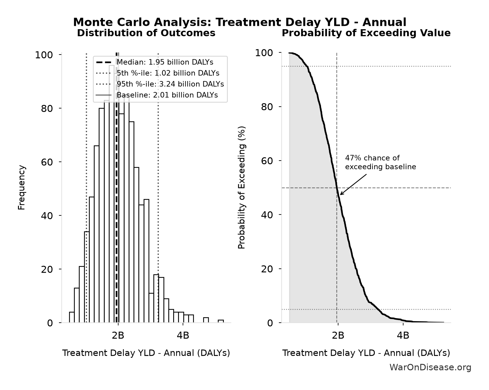
Simulation Results Summary: Treatment Delay YLD - Annual
| Statistic | Value |
|---|---|
| Baseline (deterministic) | 2.01 billion |
| Mean (expected value) | 2.02 billion |
| Median (50th percentile) | 1.95 billion |
| Standard Deviation | 682 million |
| 90% Range (5th-95th percentile) | [1.02 billion, 3.24 billion] |
The histogram shows 1,000 of the 10,000 Monte Carlo draws for Treatment Delay YLD - Annual; the summary statistics use all 10,000. The exceedance curve (right) shows the probability of the outcome exceeding any given value.
Exceedance Probability
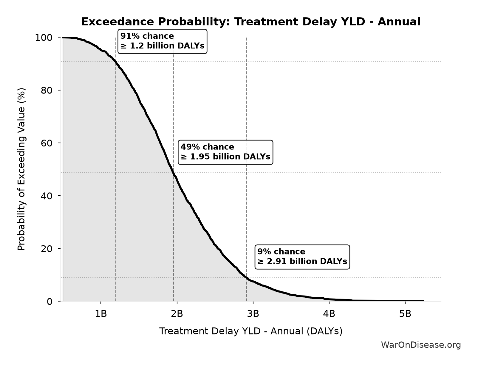
This exceedance probability chart shows the likelihood that Treatment Delay YLD - Annual will exceed any given threshold. The higher the curve at a threshold, the more likely the value exceeds it.
Total Deaths from Historical Progress Delays: 102 million deaths
Note📊 Details
Total deaths from delaying existing drugs over 8.2-year efficacy lag. One-time impact of eliminating Phase 2-4 testing delay for drugs already approved 1962-2024. Based on Lichtenberg (2019) estimate of 12M lives saved annually × 8.2 years efficacy lag. Excludes innovation acceleration effects.
Inputs:
- Annual Lives Saved by Pharmaceuticals 🔢: 12.4 million deaths
- Regulatory Delay for Efficacy Testing Post-Safety Verification 📊: 8.2 years (SE: ±2 years)
\[ \begin{gathered} Deaths_{lag,total} \\ = Lives_{saved,annual} \times T_{lag} \\ = 12.4M \times 8.2 \\ = 102M \end{gathered} \] where: \[ \begin{gathered} Lives_{saved,annual} \\ = \frac{LY_{saved,annual}}{T_{ext}} \\ = \frac{149M}{12} \\ = 12.4M \end{gathered} \] ~ Medium confidence
Sensitivity Analysis
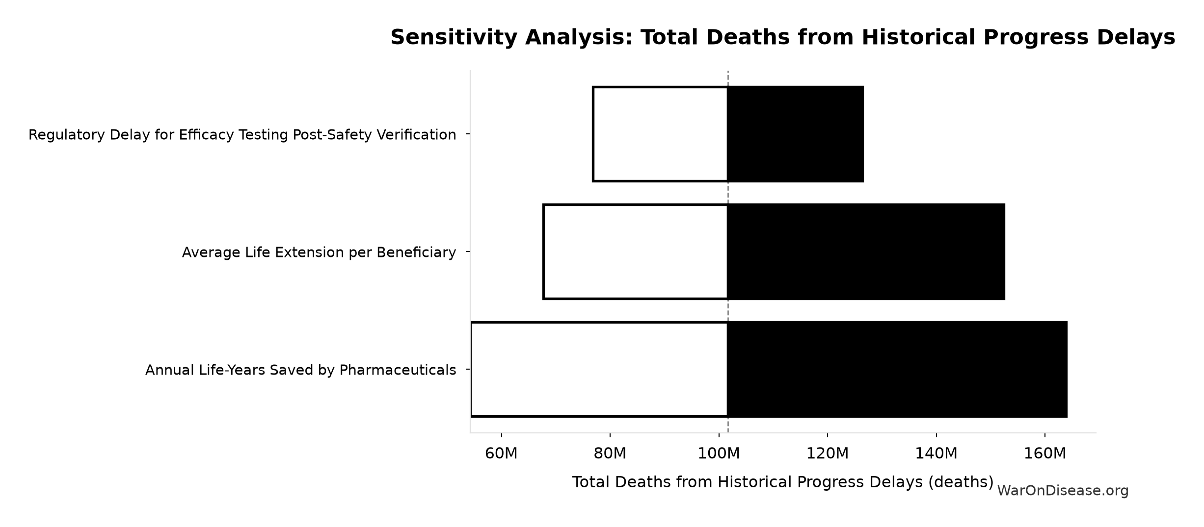
Sensitivity Indices for Total Deaths from Historical Progress Delays
Regression-based sensitivity showing which inputs explain the most variance in the output.
| Input Parameter | Sensitivity Coefficient | Interpretation |
|---|---|---|
| Annual Lives Saved by Pharmaceuticals (deaths) | 0.7195 | Strong driver |
| Regulatory Delay for Efficacy Testing Post-Safety Verification (years) | 0.6685 | Strong driver |
Interpretation: Standardized coefficients show the change in output (in SD units) per 1 SD change in input. Values near ±1 indicate strong influence; values exceeding ±1 may occur with correlated inputs.
Monte Carlo Distribution
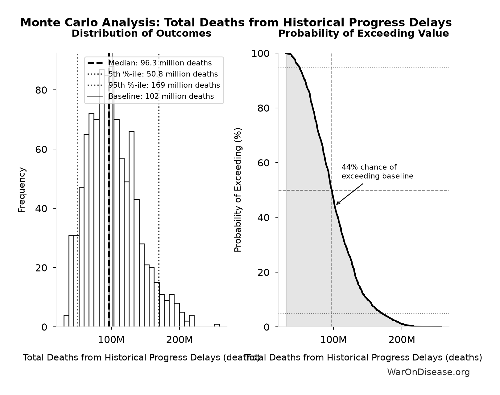
Simulation Results Summary: Total Deaths from Historical Progress Delays
| Statistic | Value |
|---|---|
| Baseline (deterministic) | 102 million |
| Mean (expected value) | 101 million |
| Median (50th percentile) | 96.3 million |
| Standard Deviation | 36.3 million |
| 90% Range (5th-95th percentile) | [50.8 million, 169 million] |
The histogram shows 1,000 of the 10,000 Monte Carlo draws for Total Deaths from Historical Progress Delays; the summary statistics use all 10,000. The exceedance curve (right) shows the probability of the outcome exceeding any given value.
Exceedance Probability
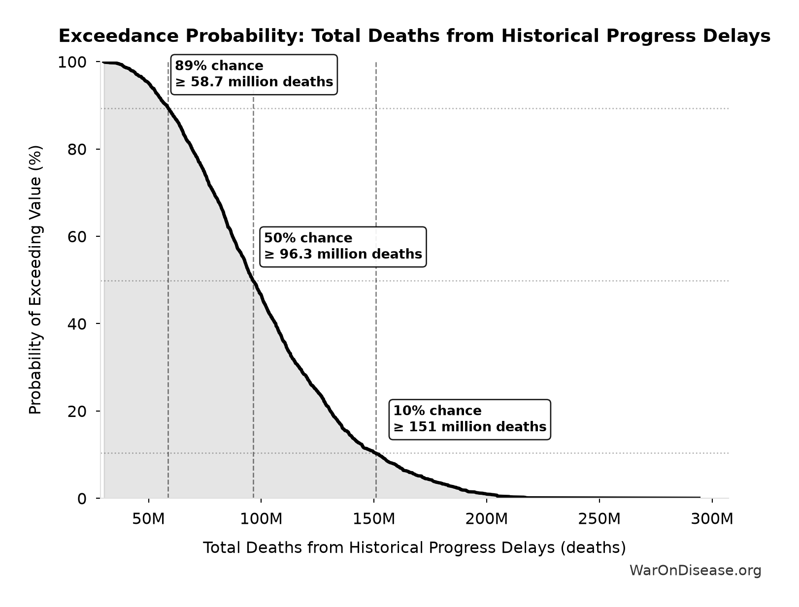
This exceedance probability chart shows the likelihood that Total Deaths from Historical Progress Delays will exceed any given threshold. The higher the curve at a threshold, the more likely the value exceeds it.
Therapeutic Frontier Exploration Ratio: 0.342%
Note📊 Details
Fraction of possible drug-disease space actually tested (<1%)
Inputs:
- Tested Drug-Disease Relationships: 32,500 relationships (95% CI: 15,000 relationships - 50,000 relationships)
- Possible Drug-Disease Combinations 🔢: 9.5 million combinations
\[ \begin{gathered} Ratio_{explore} \\ = \frac{N_{tested}}{N_{combos}} \\ = \frac{32{,}500}{9.5M} \\ = 0.342\% \end{gathered} \] where: \[ \begin{gathered} N_{combos} \\ = N_{safe} \times N_{diseases,trial} \\ = 9{,}500 \times 1{,}000 \\ = 9.5M \end{gathered} \] ✓ High confidence
Sensitivity Analysis
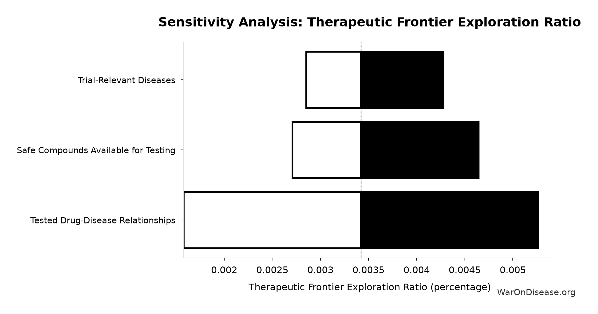
Sensitivity Indices for Therapeutic Frontier Exploration Ratio
Regression-based sensitivity showing which inputs explain the most variance in the output.
| Input Parameter | Sensitivity Coefficient | Interpretation |
|---|---|---|
| Tested Drug-Disease Relationships (relationships) | 0.7794 | Strong driver |
| Possible Drug-Disease Combinations (combinations) | -0.5916 | Strong driver |
Interpretation: Standardized coefficients show the change in output (in SD units) per 1 SD change in input. Values near ±1 indicate strong influence; values exceeding ±1 may occur with correlated inputs.
Monte Carlo Distribution
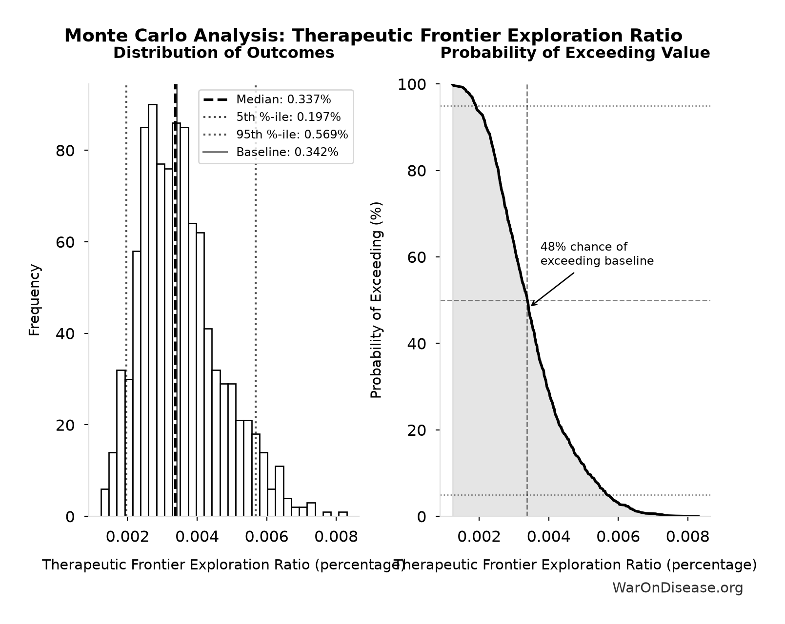
Simulation Results Summary: Therapeutic Frontier Exploration Ratio
| Statistic | Value |
|---|---|
| Baseline (deterministic) | 0.342% |
| Mean (expected value) | 0.354% |
| Median (50th percentile) | 0.337% |
| Standard Deviation | 0.116% |
| 90% Range (5th-95th percentile) | [0.197%, 0.569%] |
The histogram shows 1,000 of the 10,000 Monte Carlo draws for Therapeutic Frontier Exploration Ratio; the summary statistics use all 10,000. The exceedance curve (right) shows the probability of the outcome exceeding any given value.
Exceedance Probability
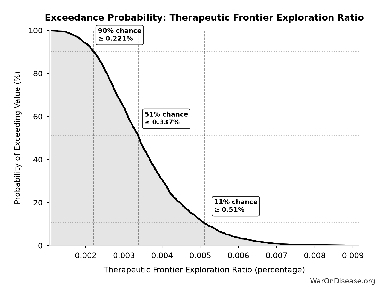
This exceedance probability chart shows the likelihood that Therapeutic Frontier Exploration Ratio will exceed any given threshold. The higher the curve at a threshold, the more likely the value exceeds it.
Annual Welfare Cost of Avoidable Disease: $400 trillion
Note📊 Details
Annual welfare cost of avoidable disease globally. Calculated as global DALY burden × eventually avoidable percentage × standard QALY value ($150K). Uses consistent QALY valuation matching all other health impact calculations. Medical costs and productivity losses are NOT added separately to avoid double-counting (QALY valuation already captures these welfare components).
Inputs:
- Global Annual DALY Burden 📊: 2.88 billion DALYs/year (SE: ±150 million DALYs/year)
- Eventually Avoidable DALY Percentage: 92.6% (95% CI: 50% - 98%)
- Standard Economic Value per QALY 📊: $150,000 (SE: ±$30,000)
\[ \begin{gathered} Burden_{disease} \\ = DALYs_{global,ann} \times Pct_{avoid,DALY} \times Value_{QALY} \\ = 2.88B \times 92.6\% \times \$150K \\ = \$400T \end{gathered} \]
✓ High confidence
Sensitivity Analysis
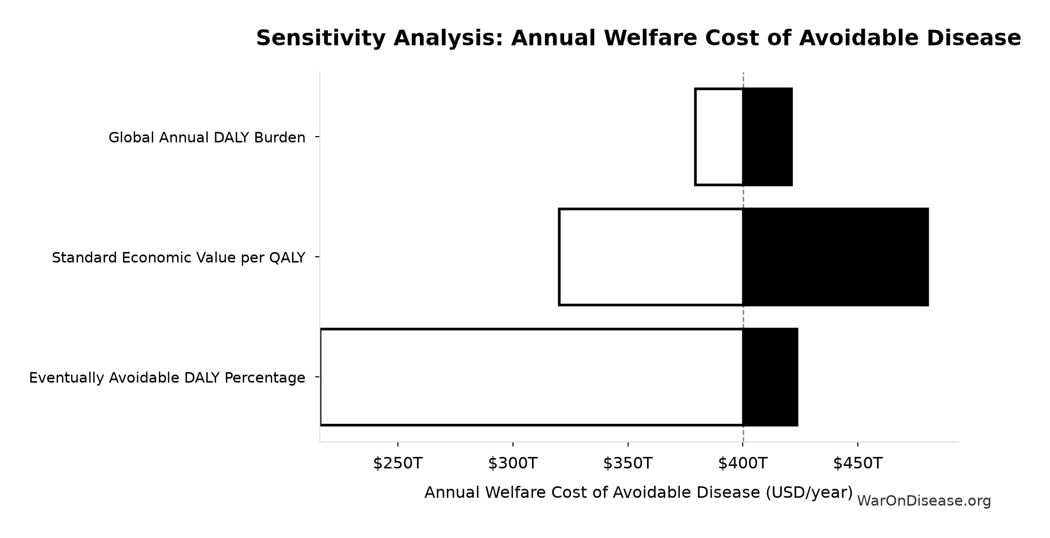
Sensitivity Indices for Annual Welfare Cost of Avoidable Disease
Regression-based sensitivity showing which inputs explain the most variance in the output.
| Input Parameter | Sensitivity Coefficient | Interpretation |
|---|---|---|
| Standard Economic Value per QALY (USD/QALY) | 0.8093 | Strong driver |
| Eventually Avoidable DALY Percentage (percentage) | 0.5200 | Strong driver |
| Global Annual DALY Burden (DALYs/year) | 0.2294 | Weak driver |
Interpretation: Standardized coefficients show the change in output (in SD units) per 1 SD change in input. Values near ±1 indicate strong influence; values exceeding ±1 may occur with correlated inputs.
Monte Carlo Distribution
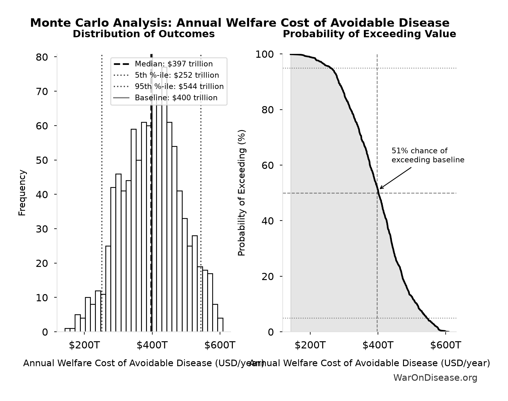
Simulation Results Summary: Annual Welfare Cost of Avoidable Disease
| Statistic | Value |
|---|---|
| Baseline (deterministic) | $400 trillion |
| Mean (expected value) | $397 trillion |
| Median (50th percentile) | $397 trillion |
| Standard Deviation | $89.5 trillion |
| 90% Range (5th-95th percentile) | [$252 trillion, $544 trillion] |
The histogram shows 1,000 of the 10,000 Monte Carlo draws for Annual Welfare Cost of Avoidable Disease; the summary statistics use all 10,000. The exceedance curve (right) shows the probability of the outcome exceeding any given value.
Exceedance Probability
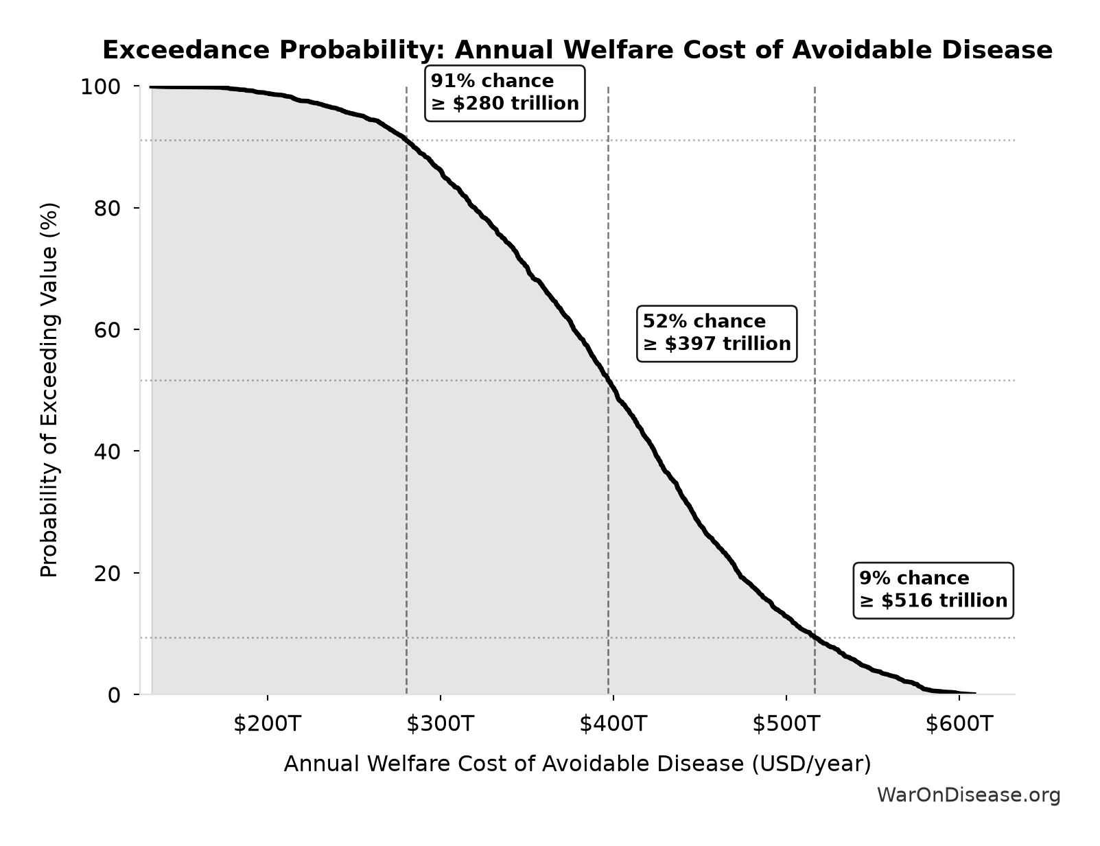
This exceedance probability chart shows the likelihood that Annual Welfare Cost of Avoidable Disease will exceed any given threshold. The higher the curve at a threshold, the more likely the value exceeds it.
Annual Lives Saved by Pharmaceuticals: 12.4 million deaths
Note📊 Details
Annual lives saved by pharmaceutical interventions globally. Derived from Lichtenberg (2019) finding of 148.7M life-years saved, divided by assumed 12-year average life extension per beneficiary. Note: Life-years is the primary metric; lives is an approximation for intuitive communication.
Inputs:
- Annual Life-Years Saved by Pharmaceuticals 📊: 149 million life-years (95% CI: 79.4 million life-years - 240 million life-years)
- Average Life Extension per Beneficiary: 12 years (95% CI: 8 years - 18 years)
\[ \begin{gathered} Lives_{saved,annual} \\ = \frac{LY_{saved,annual}}{T_{ext}} \\ = \frac{149M}{12} \\ = 12.4M \end{gathered} \]
Methodology:21
? Low confidence
Sensitivity Analysis
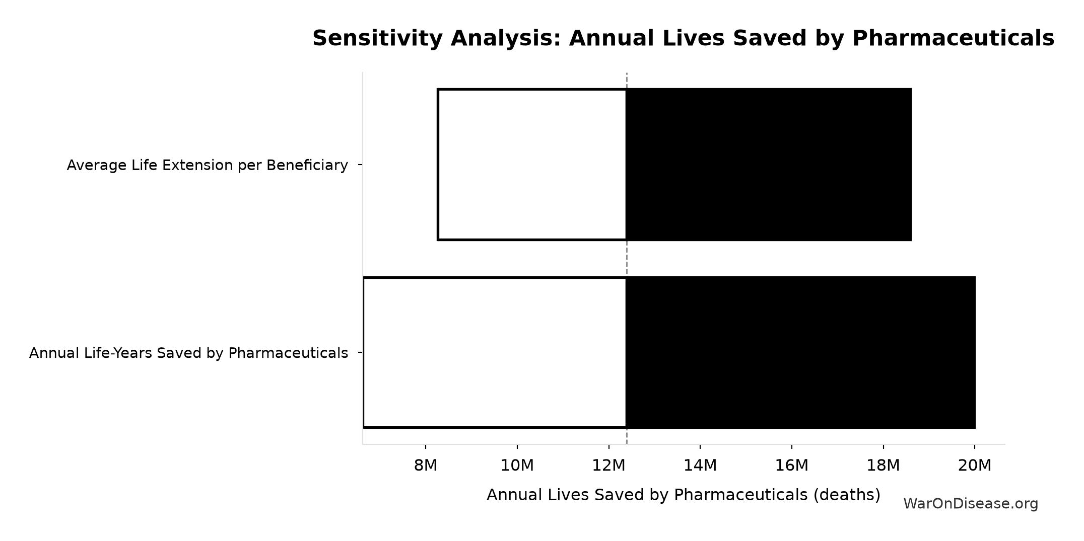
Sensitivity Indices for Annual Lives Saved by Pharmaceuticals
Regression-based sensitivity showing which inputs explain the most variance in the output.
| Input Parameter | Sensitivity Coefficient | Interpretation |
|---|---|---|
| Annual Life-Years Saved by Pharmaceuticals (life-years) | 1.0000 | Strong driver |
Interpretation: Standardized coefficients show the change in output (in SD units) per 1 SD change in input. Values near ±1 indicate strong influence; values exceeding ±1 may occur with correlated inputs.
Monte Carlo Distribution
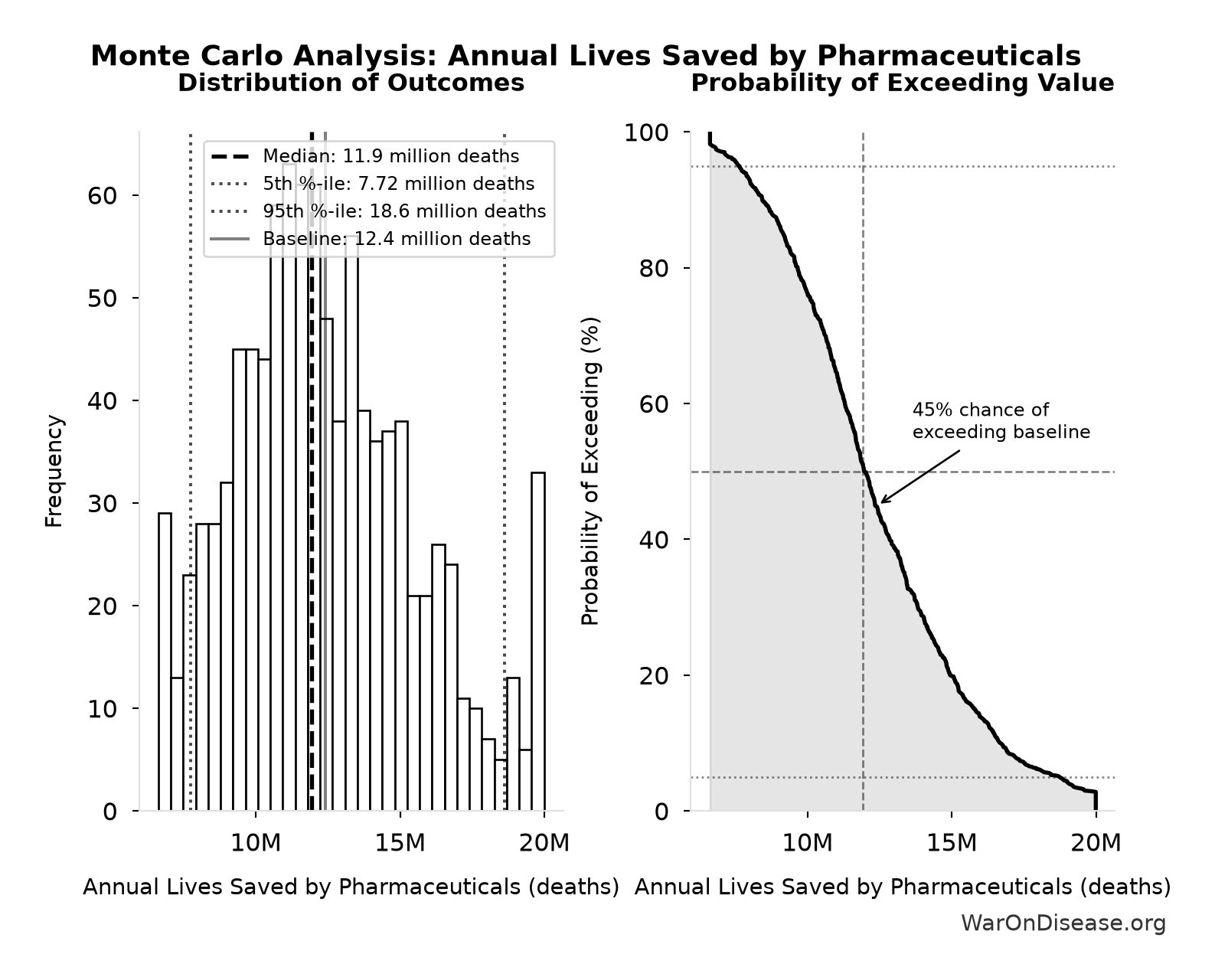
Simulation Results Summary: Annual Lives Saved by Pharmaceuticals
| Statistic | Value |
|---|---|
| Baseline (deterministic) | 12.4 million |
| Mean (expected value) | 12.3 million |
| Median (50th percentile) | 11.9 million |
| Standard Deviation | 3.17 million |
| 90% Range (5th-95th percentile) | [7.72 million, 18.6 million] |
The histogram shows 1,000 of the 10,000 Monte Carlo draws for Annual Lives Saved by Pharmaceuticals; the summary statistics use all 10,000. The exceedance curve (right) shows the probability of the outcome exceeding any given value.
Exceedance Probability
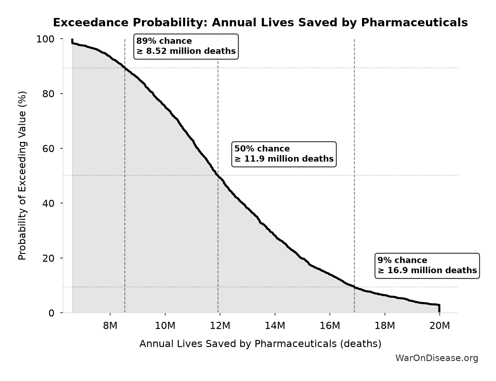
This exceedance probability chart shows the likelihood that Annual Lives Saved by Pharmaceuticals will exceed any given threshold. The higher the curve at a threshold, the more likely the value exceeds it.
Pragmatic Trial Cost per QALY (RECOVERY): $4
Note📊 Details
Cost per QALY for pragmatic platform trials, calculated from RECOVERY trial data. Uses global impact methodology: trial cost divided by total QALYs from downstream adoption. This measures research efficiency (discovery value), not clinical intervention ICER.
Inputs:
- RECOVERY Trial Total Cost 📊: $20 million (95% CI: $15 million - $25 million)
- RECOVERY Trial Total QALYs Generated 🔢: 5 million QALYs
\[ \begin{gathered} Cost_{pragmatic,QALY} \\ = \frac{Cost_{RECOVERY}}{QALY_{RECOVERY}} \\ = \frac{\$20M}{5M} \\ = \$4 \end{gathered} \] where: \[ \begin{gathered} QALY_{RECOVERY} \\ = Lives_{RECOVERY} \times QALY_{COVID} \\ = 1M \times 5 \\ = 5M \end{gathered} \] Methodology:31
~ Medium confidence
Sensitivity Analysis
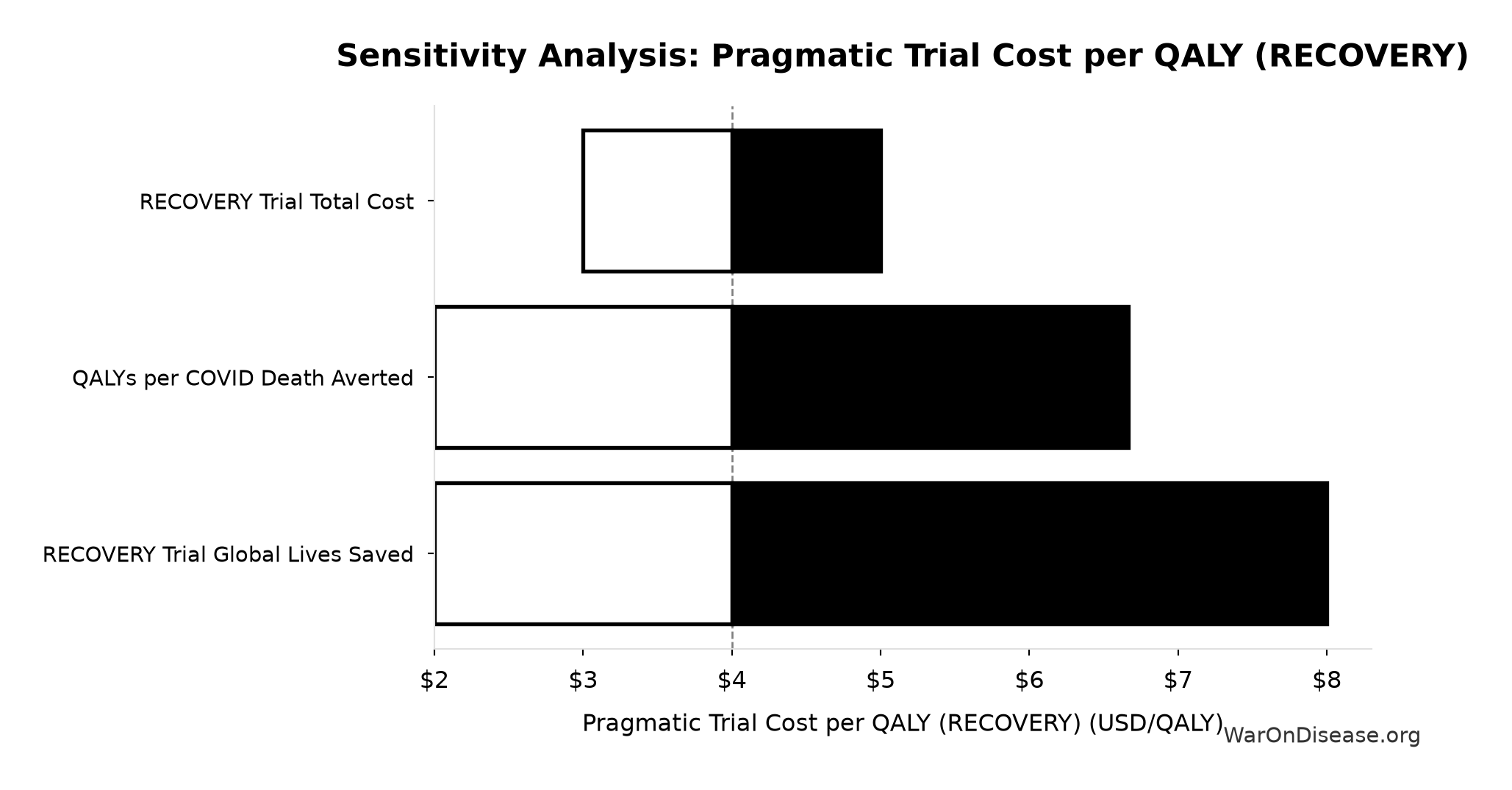
Sensitivity Indices for Pragmatic Trial Cost per QALY (RECOVERY)
Regression-based sensitivity showing which inputs explain the most variance in the output.
| Input Parameter | Sensitivity Coefficient | Interpretation |
|---|---|---|
| RECOVERY Trial Total QALYs Generated (QALYs) | -0.7945 | Strong driver |
| RECOVERY Trial Total Cost (USD) | 0.2519 | Weak driver |
Interpretation: Standardized coefficients show the change in output (in SD units) per 1 SD change in input. Values near ±1 indicate strong influence; values exceeding ±1 may occur with correlated inputs.
Monte Carlo Distribution
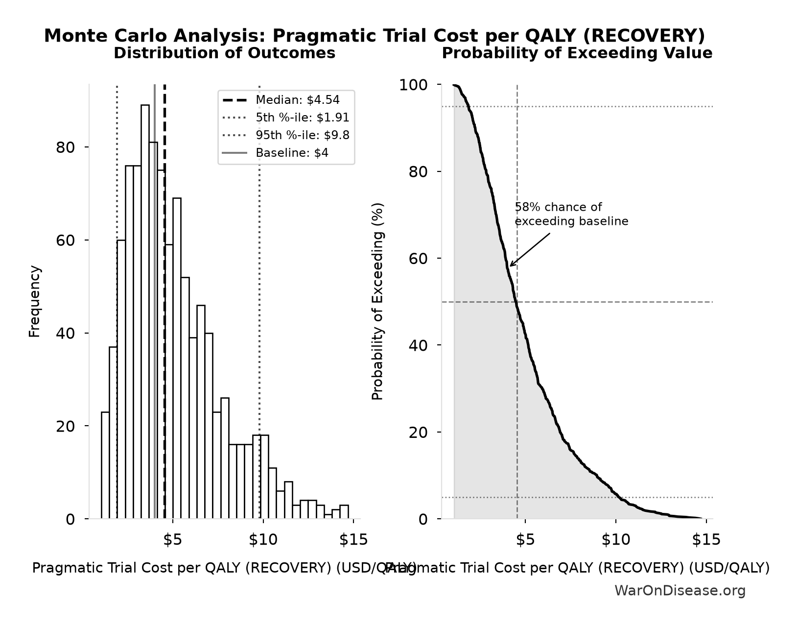
Simulation Results Summary: Pragmatic Trial Cost per QALY (RECOVERY)
| Statistic | Value |
|---|---|
| Baseline (deterministic) | $4 |
| Mean (expected value) | $5.03 |
| Median (50th percentile) | $4.54 |
| Standard Deviation | $2.47 |
| 90% Range (5th-95th percentile) | [$1.91, $9.8] |
The histogram shows 1,000 of the 10,000 Monte Carlo draws for Pragmatic Trial Cost per QALY (RECOVERY); the summary statistics use all 10,000. The exceedance curve (right) shows the probability of the outcome exceeding any given value.
Exceedance Probability
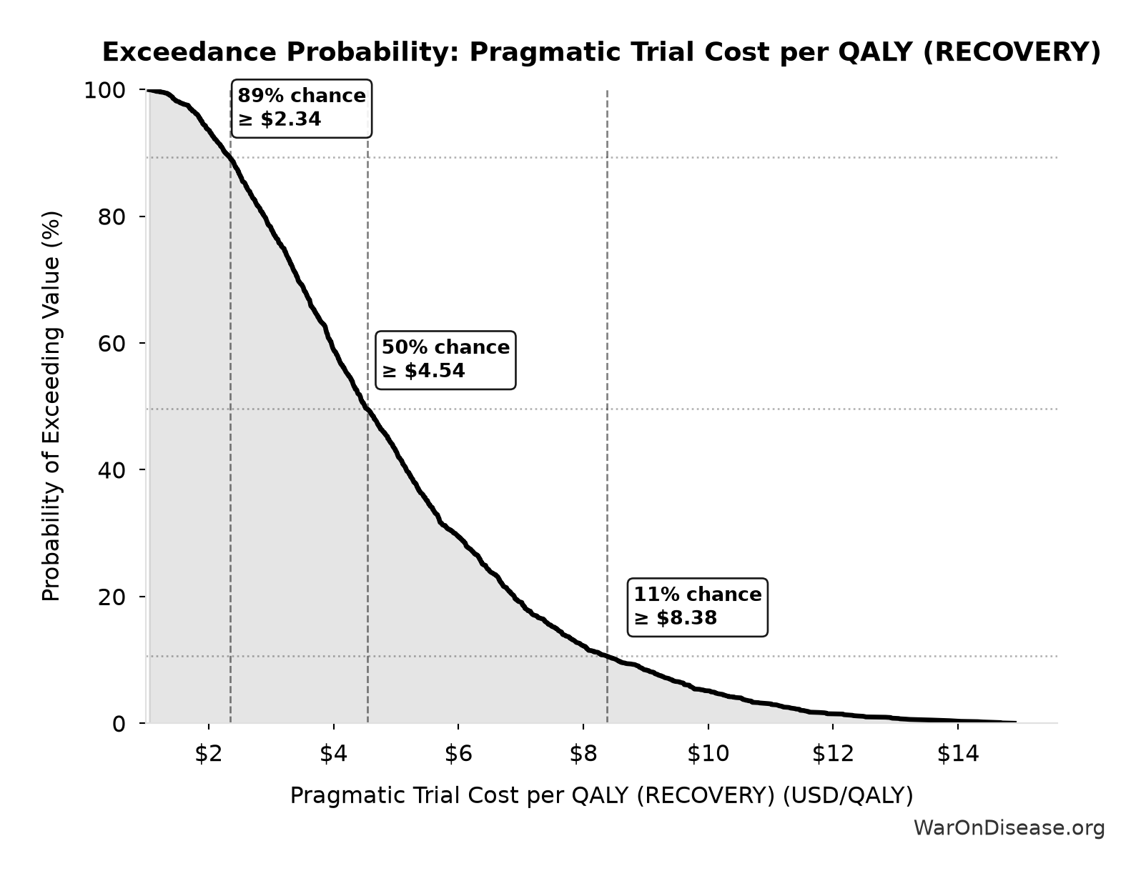
This exceedance probability chart shows the likelihood that Pragmatic Trial Cost per QALY (RECOVERY) will exceed any given threshold. The higher the curve at a threshold, the more likely the value exceeds it.
RECOVERY Trial Cost Reduction Factor: 82x
Note📊 Details
Cost reduction factor demonstrated by RECOVERY trial (traditional Phase 3 cost / RECOVERY cost per patient)
Inputs:
- Phase 3 Cost per Patient 📊: $41,000 (95% CI: $20,000 - $120,000)
- Recovery Trial Cost per Patient 📊: $500 (95% CI: $400 - $2,500)
\[ \begin{gathered} k_{RECOVERY} \\ = \frac{Cost_{P3,pt}}{Cost_{RECOVERY,pt}} \\ = \frac{\$41K}{\$500} \\ = 82 \end{gathered} \]
Methodology:31
✓ High confidence
Sensitivity Analysis
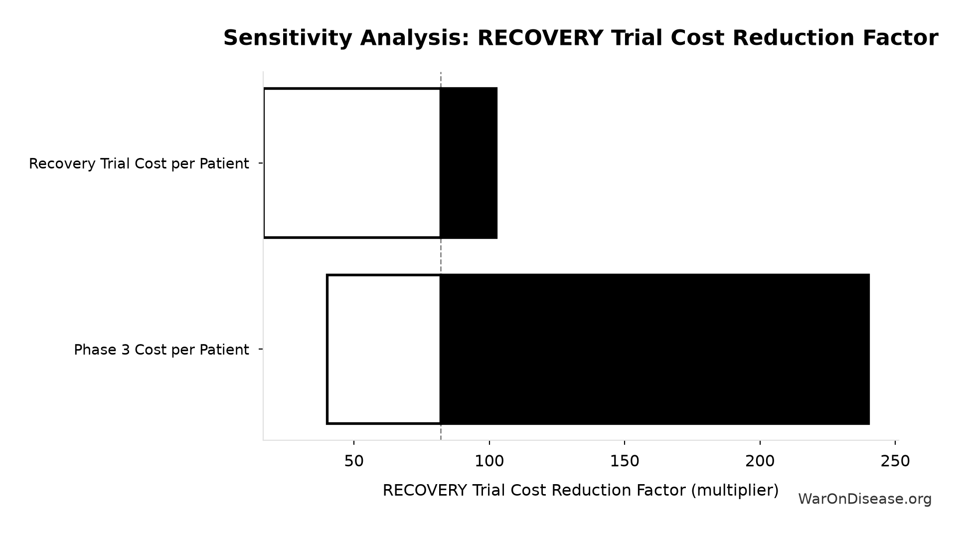
Sensitivity Indices for RECOVERY Trial Cost Reduction Factor
Regression-based sensitivity showing which inputs explain the most variance in the output.
| Input Parameter | Sensitivity Coefficient | Interpretation |
|---|---|---|
| Phase 3 Cost per Patient (USD/patient) | 0.8407 | Strong driver |
| Recovery Trial Cost per Patient (USD/patient) | -0.4419 | Moderate driver |
Interpretation: Standardized coefficients show the change in output (in SD units) per 1 SD change in input. Values near ±1 indicate strong influence; values exceeding ±1 may occur with correlated inputs.
Monte Carlo Distribution
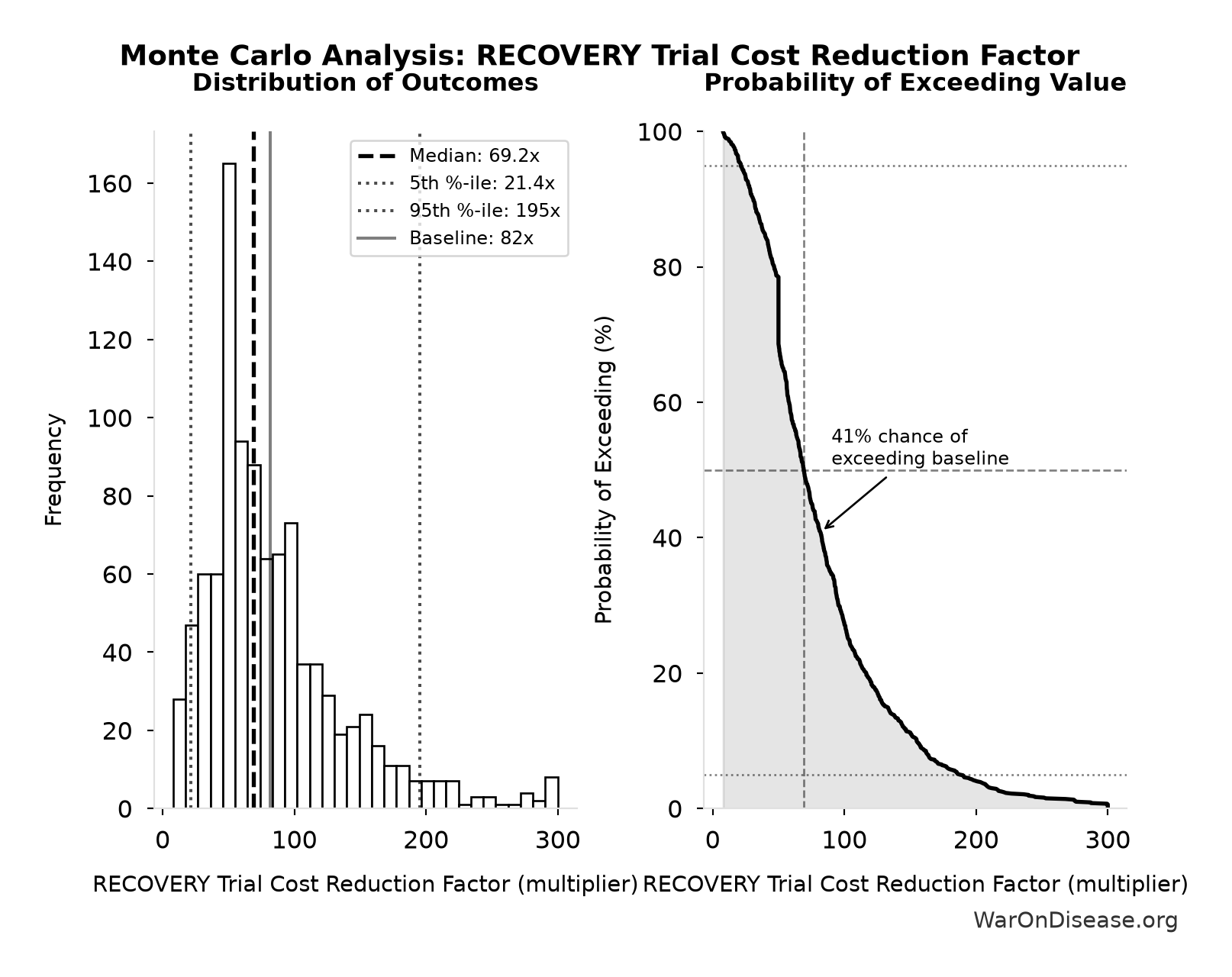
Simulation Results Summary: RECOVERY Trial Cost Reduction Factor
| Statistic | Value |
|---|---|
| Baseline (deterministic) | 82x |
| Mean (expected value) | 84.2x |
| Median (50th percentile) | 69.2x |
| Standard Deviation | 54.5x |
| 90% Range (5th-95th percentile) | [21.4x, 195x] |
The histogram shows 1,000 of the 10,000 Monte Carlo draws for RECOVERY Trial Cost Reduction Factor; the summary statistics use all 10,000. The exceedance curve (right) shows the probability of the outcome exceeding any given value.
Exceedance Probability
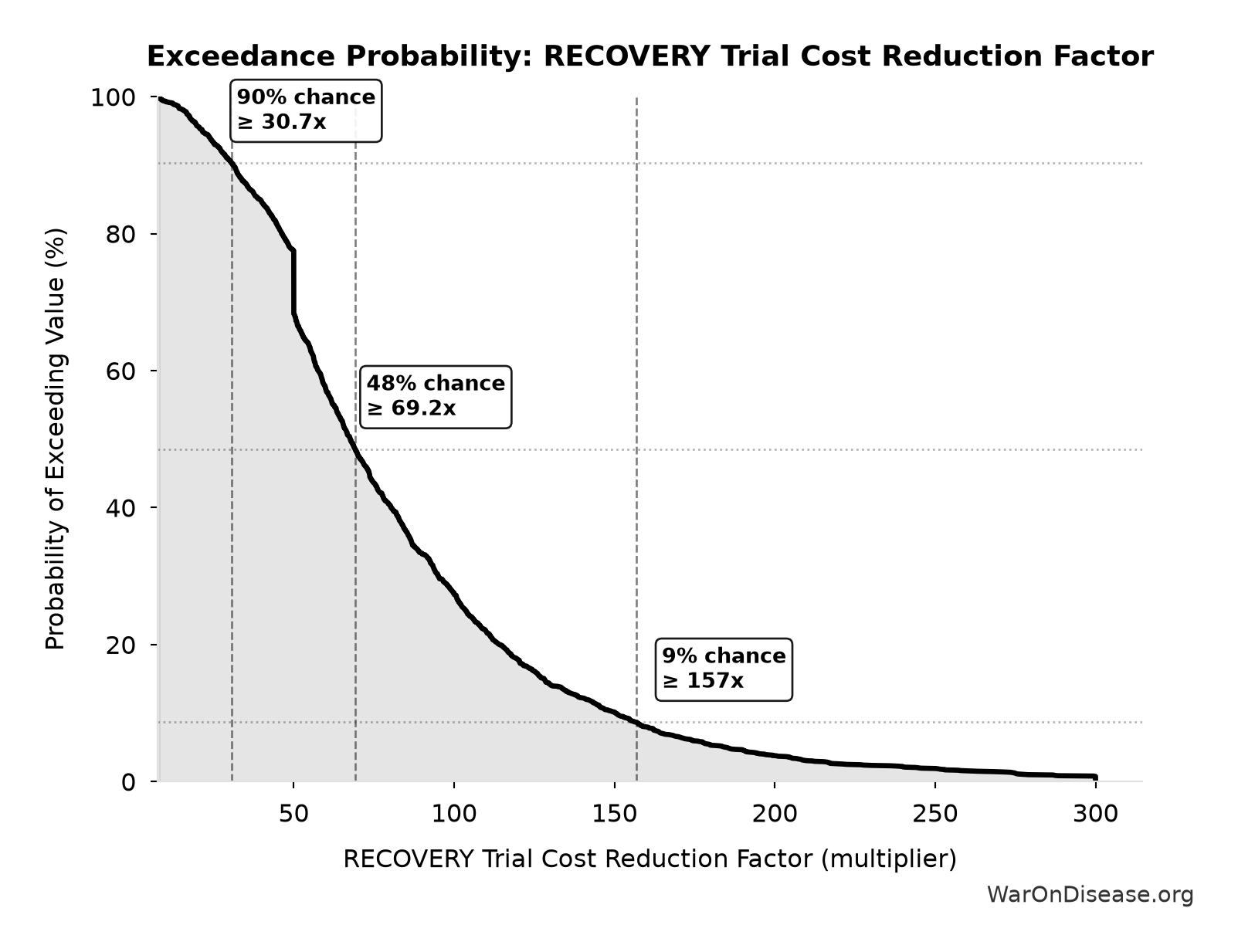
This exceedance probability chart shows the likelihood that RECOVERY Trial Cost Reduction Factor will exceed any given threshold. The higher the curve at a threshold, the more likely the value exceeds it.
RECOVERY Trial Total QALYs Generated: 5 million QALYs
Note📊 Details
Total QALYs generated by RECOVERY trial’s discoveries (lives saved × QALYs per life). Uses global impact methodology: counts all downstream health gains from the discovery.
Inputs:
- RECOVERY Trial Global Lives Saved 📊: 1 million lives (95% CI: 500 thousand lives - 2 million lives)
- QALYs per COVID Death Averted: 5 QALYs/death (95% CI: 3 QALYs/death - 10 QALYs/death)
\[ \begin{gathered} QALY_{RECOVERY} \\ = Lives_{RECOVERY} \times QALY_{COVID} \\ = 1M \times 5 \\ = 5M \end{gathered} \]
~ Medium confidence
Sensitivity Analysis
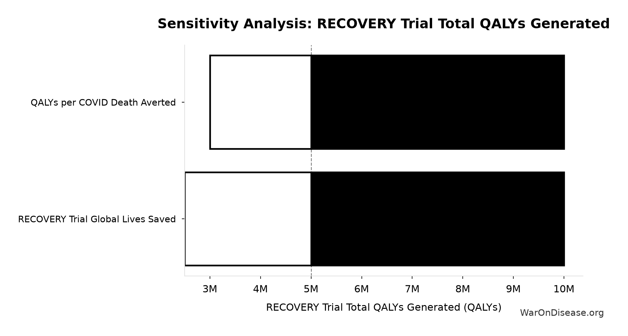
Sensitivity Indices for RECOVERY Trial Total QALYs Generated
Regression-based sensitivity showing which inputs explain the most variance in the output.
| Input Parameter | Sensitivity Coefficient | Interpretation |
|---|---|---|
| RECOVERY Trial Global Lives Saved (lives) | 0.7055 | Strong driver |
| QALYs per COVID Death Averted (QALYs/death) | 0.6520 | Strong driver |
Interpretation: Standardized coefficients show the change in output (in SD units) per 1 SD change in input. Values near ±1 indicate strong influence; values exceeding ±1 may occur with correlated inputs.
Monte Carlo Distribution
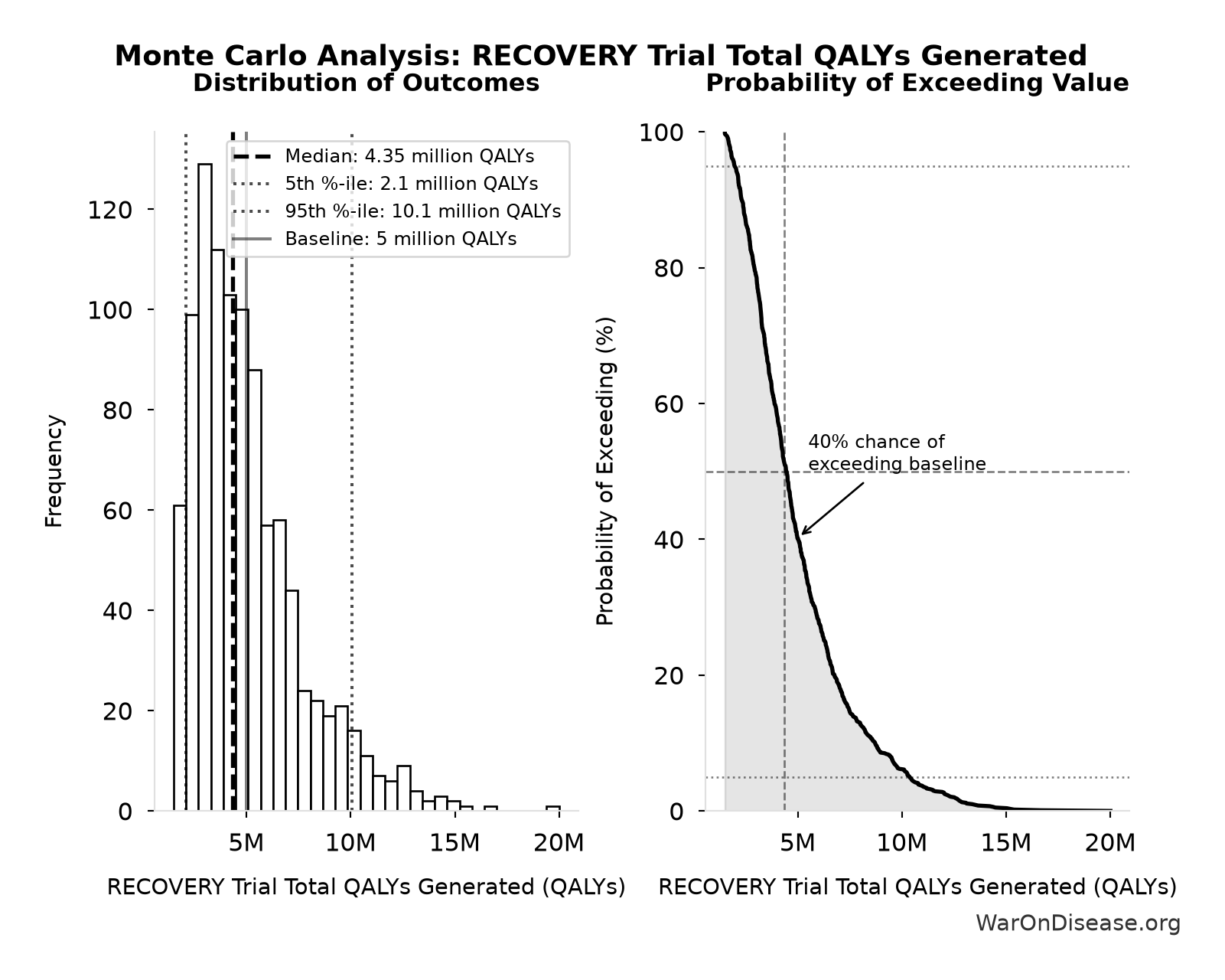
Simulation Results Summary: RECOVERY Trial Total QALYs Generated
| Statistic | Value |
|---|---|
| Baseline (deterministic) | 5 million |
| Mean (expected value) | 4.97 million |
| Median (50th percentile) | 4.35 million |
| Standard Deviation | 2.53 million |
| 90% Range (5th-95th percentile) | [2.1 million, 10.1 million] |
The histogram shows 1,000 of the 10,000 Monte Carlo draws for RECOVERY Trial Total QALYs Generated; the summary statistics use all 10,000. The exceedance curve (right) shows the probability of the outcome exceeding any given value.
Exceedance Probability
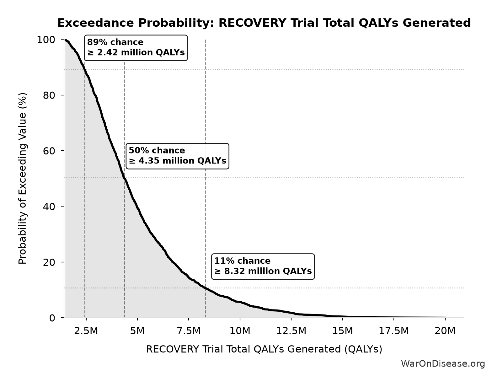
This exceedance probability chart shows the likelihood that RECOVERY Trial Total QALYs Generated will exceed any given threshold. The higher the curve at a threshold, the more likely the value exceeds it.
Universal Right to Try with Evidence Implementation Cost per DALY: $0.000134
Note📊 Details
Conditional implementation cost per DALY if all 50 states adopt, a mature pooled pragmatic-trial system operates under applicable federal authorization, and the modeled treatment-discovery acceleration occurs. The numerator includes the 50-state campaign and ten-year registry launch costs, excludes patient or payer spending on treatment delivery, trial-site services, and permitted study costs, and assumes center assessments fund the registry thereafter. The denominator counts the global treatment schedule shift once.
Inputs:
- Universal Right to Try with Evidence Implementation Cost: $65 million (95% CI: $25 million - $200 million)
- DALYs Averted from Universal Right to Try with Evidence 🔢: 483 billion DALYs
\[ \begin{gathered} Cost_{RTT,DALY} \\ = \frac{C_{RTT}}{DALYs_{RTT}} \\ = \frac{\$65M}{483B} \\ = \$0.000134 \end{gathered} \] where: \[ \begin{gathered} DALYs_{RTT} \\ = DALYs_{global,ann} \times Pct_{avoid,DALY} \times T_{accel,RTT} \\ = 2.88B \times 92.6\% \times 181 \\ = 483B \end{gathered} \] where: \[ \begin{gathered} T_{accel,RTT} \\ = T_{first,SQ} \times \left(1 - \frac{1}{k_{RTT}}\right) \\ = 222 \times \left(1 - \frac{1}{5.48}\right) \\ = 181 \end{gathered} \] where: \[ \begin{gathered} T_{first,SQ} \\ = T_{queue,SQ} \times 0.5 \\ = 443 \times 0.5 \\ = 222 \end{gathered} \] where: \[ \begin{gathered} T_{queue,SQ} \\ = \frac{N_{untreated}}{Treatments_{new,ann}} \\ = \frac{6{,}650}{15} \\ = 443 \end{gathered} \] where: \[ \begin{gathered} N_{untreated} \\ = N_{rare} \times 0.95 \\ = 7{,}000 \times 0.95 \\ = 6{,}650 \end{gathered} \] ? Low confidence
Sensitivity Analysis
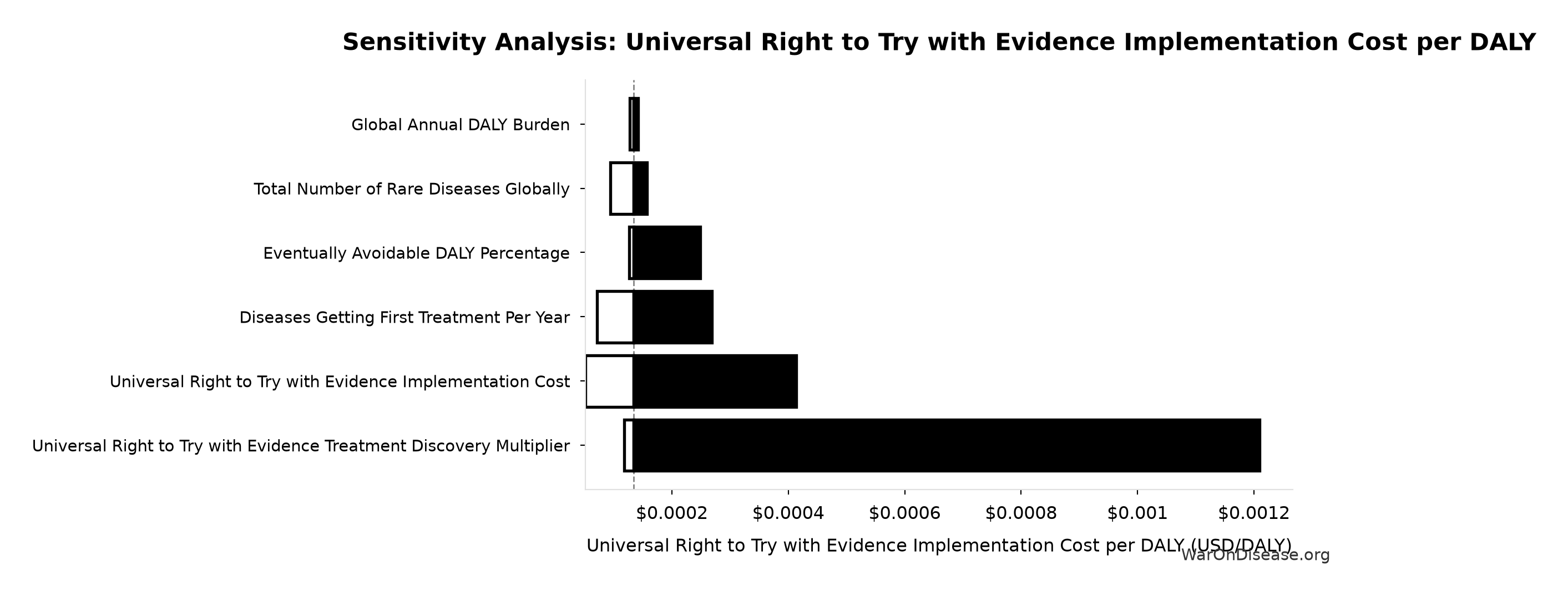
Sensitivity Indices for Universal Right to Try with Evidence Implementation Cost per DALY
Regression-based sensitivity showing which inputs explain the most variance in the output.
| Input Parameter | Sensitivity Coefficient | Interpretation |
|---|---|---|
| Universal Right to Try with Evidence Implementation Cost (USD) | 0.5492 | Strong driver |
| DALYs Averted from Universal Right to Try with Evidence (DALYs) | -0.4637 | Moderate driver |
Interpretation: Standardized coefficients show the change in output (in SD units) per 1 SD change in input. Values near ±1 indicate strong influence; values exceeding ±1 may occur with correlated inputs.
Monte Carlo Distribution
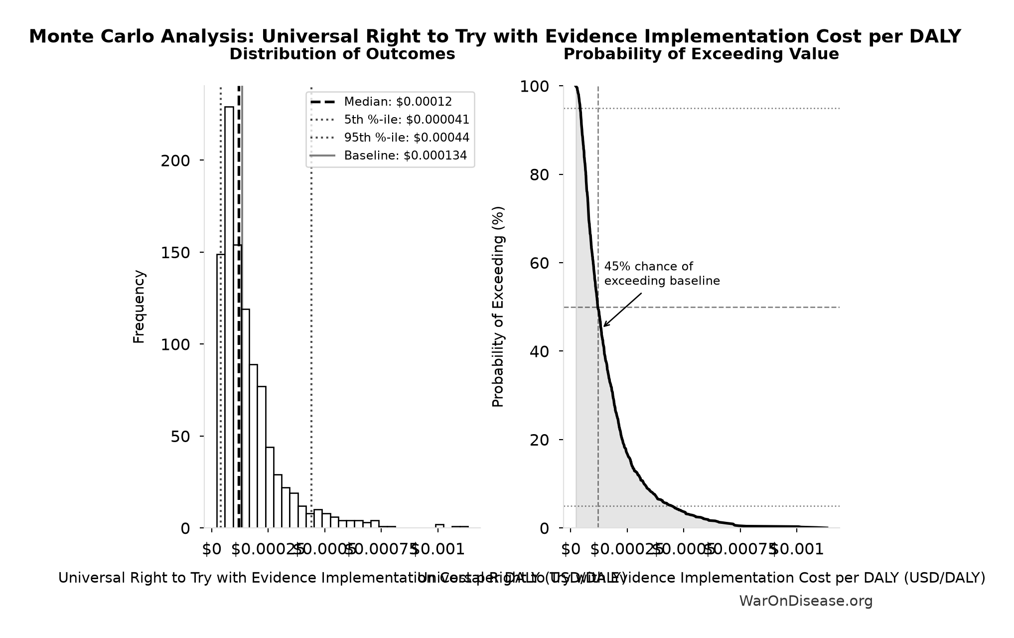
Simulation Results Summary: Universal Right to Try with Evidence Implementation Cost per DALY
| Statistic | Value |
|---|---|
| Baseline (deterministic) | $0.000134 |
| Mean (expected value) | $0.000169 |
| Median (50th percentile) | $0.00012 |
| Standard Deviation | $0.000183 |
| 90% Range (5th-95th percentile) | [$0.000041, $0.00044] |
The histogram shows 1,000 of the 10,000 Monte Carlo draws for Universal Right to Try with Evidence Implementation Cost per DALY; the summary statistics use all 10,000. The exceedance curve (right) shows the probability of the outcome exceeding any given value.
Exceedance Probability
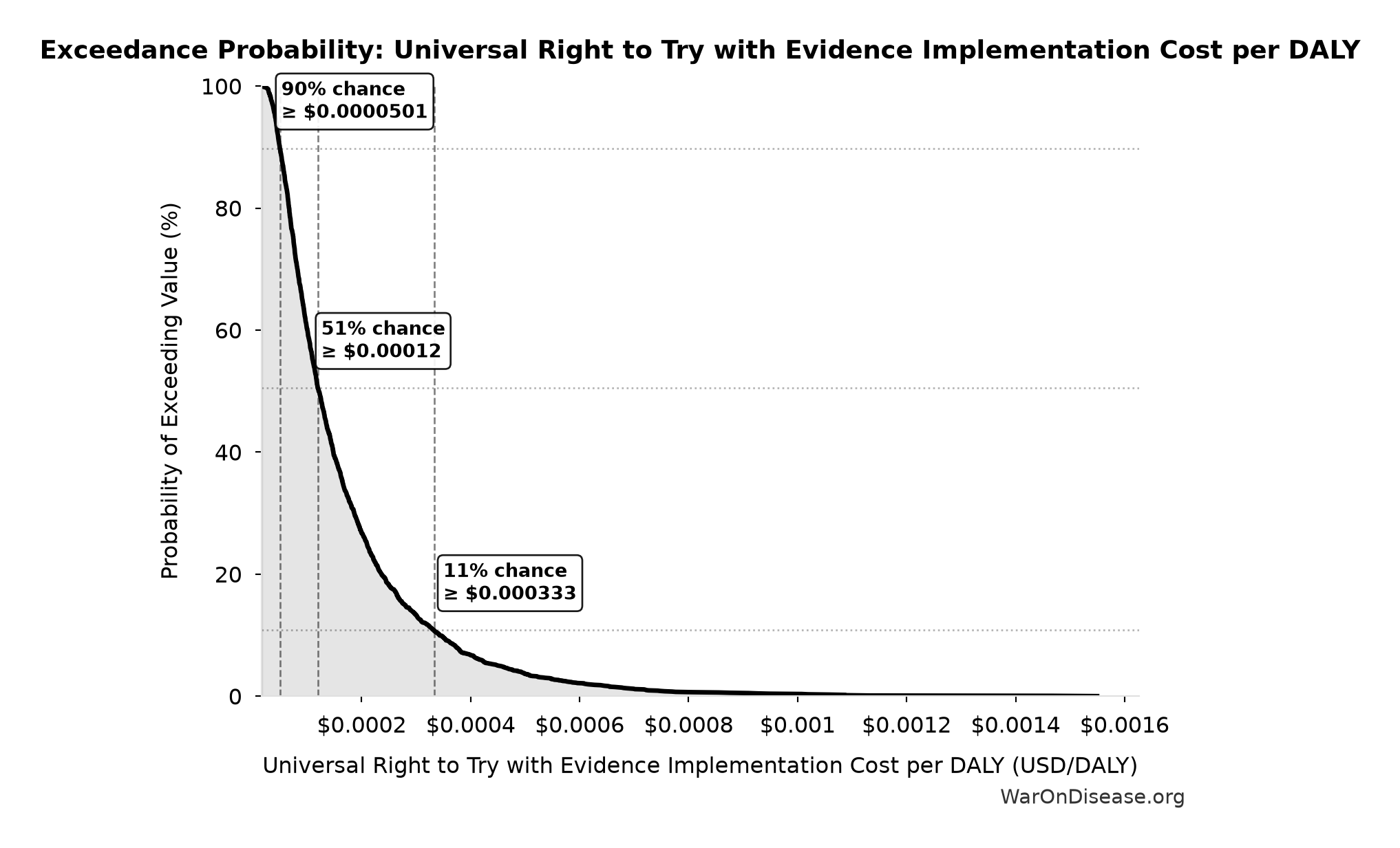
This exceedance probability chart shows the likelihood that Universal Right to Try with Evidence Implementation Cost per DALY will exceed any given threshold. The higher the curve at a threshold, the more likely the value exceeds it.
Universal Right to Try with Evidence Implementation Cost per Life Saved: $0.00707
Note📊 Details
Conditional implementation cost per modeled premature death prevented if all 50 states adopt, a mature pooled pragmatic-trial system operates, and the modeled treatment-discovery acceleration occurs. This uses the same campaign and registry numerator as the cost-per-DALY estimate.
Inputs:
- Universal Right to Try with Evidence Implementation Cost: $65 million (95% CI: $25 million - $200 million)
- Lives Saved from Universal Right to Try with Evidence 🔢: 9.19 billion deaths
\[ \begin{gathered} Cost_{RTT,life} \\ = \frac{C_{RTT}}{Lives_{RTT}} \\ = \frac{\$65M}{9.19B} \\ = \$0.00707 \end{gathered} \] where: \[ \begin{gathered} Lives_{RTT} \\ = Deaths_{disease,daily} \times Pct_{avoid,death} \times T_{accel,RTT} \times 365 \\ = 150{,}000 \times 92.6\% \times 181 \times 365 \\ = 9.19B \end{gathered} \] where: \[ \begin{gathered} T_{accel,RTT} \\ = T_{first,SQ} \times \left(1 - \frac{1}{k_{RTT}}\right) \\ = 222 \times \left(1 - \frac{1}{5.48}\right) \\ = 181 \end{gathered} \] where: \[ \begin{gathered} T_{first,SQ} \\ = T_{queue,SQ} \times 0.5 \\ = 443 \times 0.5 \\ = 222 \end{gathered} \] where: \[ \begin{gathered} T_{queue,SQ} \\ = \frac{N_{untreated}}{Treatments_{new,ann}} \\ = \frac{6{,}650}{15} \\ = 443 \end{gathered} \] where: \[ \begin{gathered} N_{untreated} \\ = N_{rare} \times 0.95 \\ = 7{,}000 \times 0.95 \\ = 6{,}650 \end{gathered} \] ? Low confidence
Sensitivity Analysis
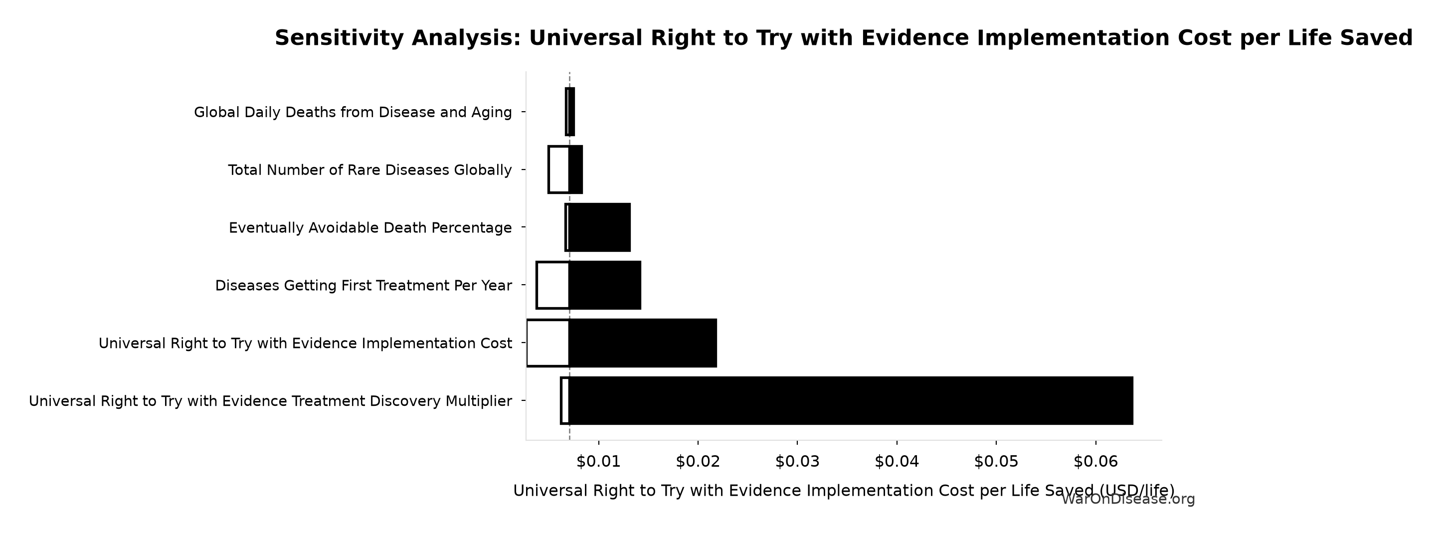
Sensitivity Indices for Universal Right to Try with Evidence Implementation Cost per Life Saved
Regression-based sensitivity showing which inputs explain the most variance in the output.
| Input Parameter | Sensitivity Coefficient | Interpretation |
|---|---|---|
| Universal Right to Try with Evidence Implementation Cost (USD) | 0.5433 | Strong driver |
| Lives Saved from Universal Right to Try with Evidence (deaths) | -0.4669 | Moderate driver |
Interpretation: Standardized coefficients show the change in output (in SD units) per 1 SD change in input. Values near ±1 indicate strong influence; values exceeding ±1 may occur with correlated inputs.
Monte Carlo Distribution
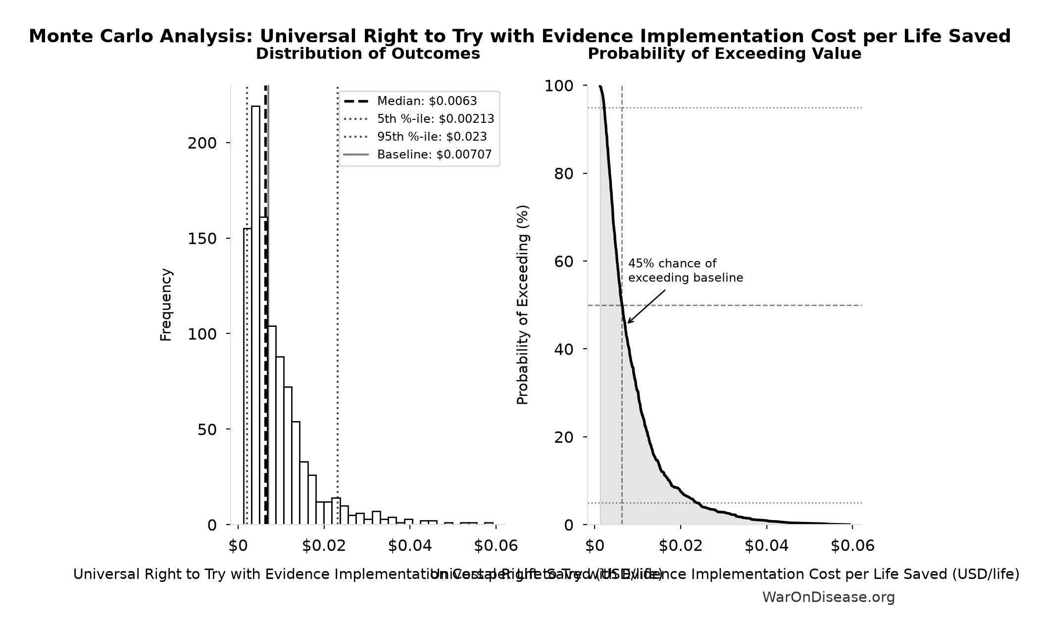
Simulation Results Summary: Universal Right to Try with Evidence Implementation Cost per Life Saved
| Statistic | Value |
|---|---|
| Baseline (deterministic) | $0.00707 |
| Mean (expected value) | $0.00892 |
| Median (50th percentile) | $0.0063 |
| Standard Deviation | $0.00973 |
| 90% Range (5th-95th percentile) | [$0.00213, $0.023] |
The histogram shows 1,000 of the 10,000 Monte Carlo draws for Universal Right to Try with Evidence Implementation Cost per Life Saved; the summary statistics use all 10,000. The exceedance curve (right) shows the probability of the outcome exceeding any given value.
Exceedance Probability
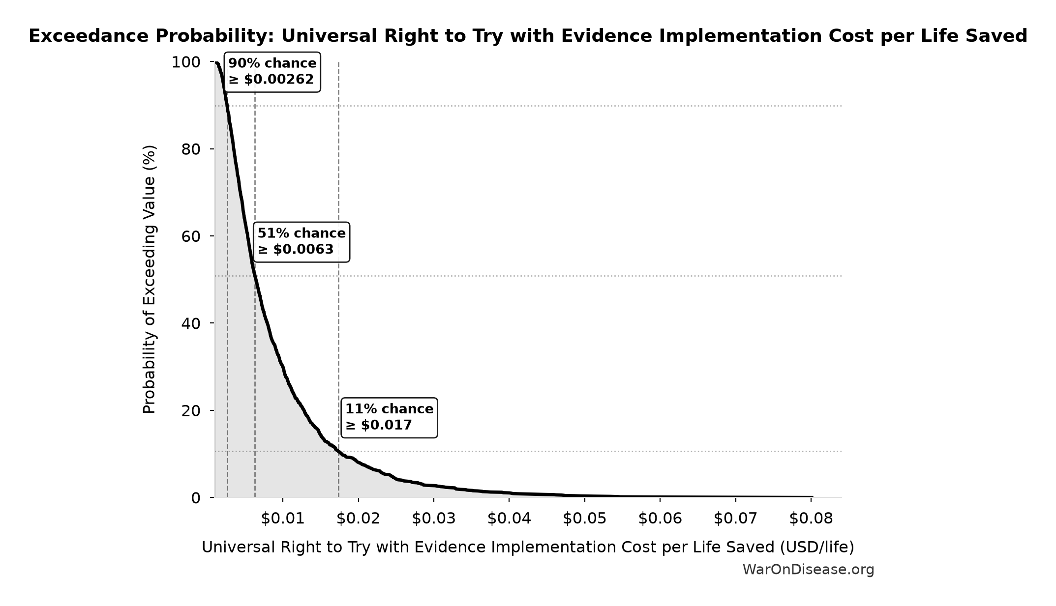
This exceedance probability chart shows the likelihood that Universal Right to Try with Evidence Implementation Cost per Life Saved will exceed any given threshold. The higher the curve at a threshold, the more likely the value exceeds it.
DALYs Averted from Universal Right to Try with Evidence: 483 billion DALYs
Note📊 Details
Conditional lifetime DALYs averted by shifting the global treatment-discovery schedule forward. By design, this applies the therapeutic-discovery timeline proxy to the eventually avoidable burden of all global diseases and aging-related degeneration. It is a schedule-shift calculation across future generations, not an observed epidemiological forecast.
Inputs:
- Global Annual DALY Burden 📊: 2.88 billion DALYs/year (SE: ±150 million DALYs/year)
- Eventually Avoidable DALY Percentage: 92.6% (95% CI: 50% - 98%)
- Average Treatment Acceleration from Universal Right to Try with Evidence 🔢: 181 years
\[ \begin{gathered} DALYs_{RTT} \\ = DALYs_{global,ann} \times Pct_{avoid,DALY} \times T_{accel,RTT} \\ = 2.88B \times 92.6\% \times 181 \\ = 483B \end{gathered} \] where: \[ \begin{gathered} T_{accel,RTT} \\ = T_{first,SQ} \times \left(1 - \frac{1}{k_{RTT}}\right) \\ = 222 \times \left(1 - \frac{1}{5.48}\right) \\ = 181 \end{gathered} \] where: \[ \begin{gathered} T_{first,SQ} \\ = T_{queue,SQ} \times 0.5 \\ = 443 \times 0.5 \\ = 222 \end{gathered} \] where: \[ \begin{gathered} T_{queue,SQ} \\ = \frac{N_{untreated}}{Treatments_{new,ann}} \\ = \frac{6{,}650}{15} \\ = 443 \end{gathered} \] where: \[ \begin{gathered} N_{untreated} \\ = N_{rare} \times 0.95 \\ = 7{,}000 \times 0.95 \\ = 6{,}650 \end{gathered} \] ? Low confidence
Sensitivity Analysis
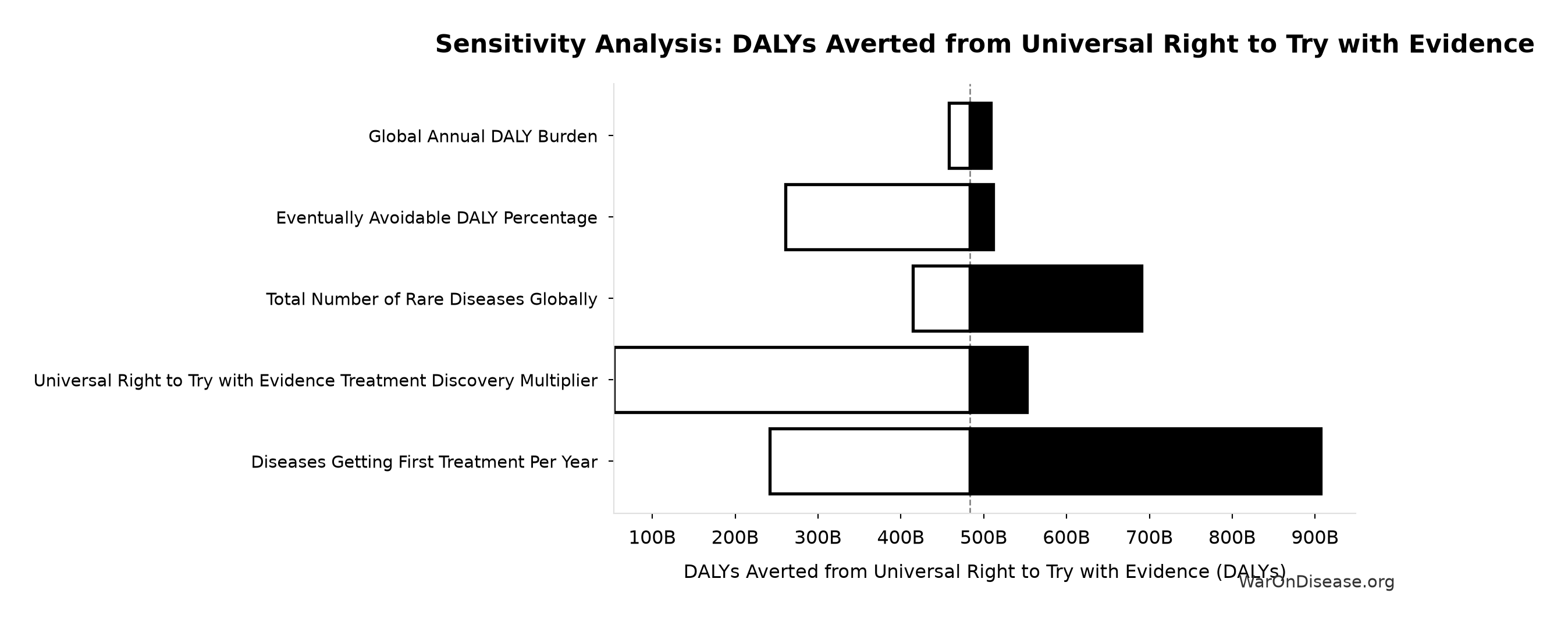
Sensitivity Indices for DALYs Averted from Universal Right to Try with Evidence
Regression-based sensitivity showing which inputs explain the most variance in the output.
| Input Parameter | Sensitivity Coefficient | Interpretation |
|---|---|---|
| Average Treatment Acceleration from Universal Right to Try with Evidence (years) | 0.9488 | Strong driver |
| Eventually Avoidable DALY Percentage (percentage) | 0.2682 | Weak driver |
| Global Annual DALY Burden (DALYs/year) | 0.1167 | Weak driver |
Interpretation: Standardized coefficients show the change in output (in SD units) per 1 SD change in input. Values near ±1 indicate strong influence; values exceeding ±1 may occur with correlated inputs.
Monte Carlo Distribution
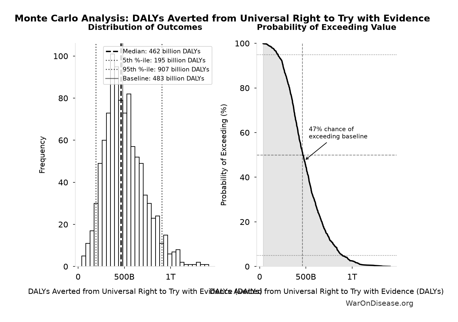
Simulation Results Summary: DALYs Averted from Universal Right to Try with Evidence
| Statistic | Value |
|---|---|
| Baseline (deterministic) | 483 billion |
| Mean (expected value) | 495 billion |
| Median (50th percentile) | 462 billion |
| Standard Deviation | 217 billion |
| 90% Range (5th-95th percentile) | [195 billion, 907 billion] |
The histogram shows 1,000 of the 10,000 Monte Carlo draws for DALYs Averted from Universal Right to Try with Evidence; the summary statistics use all 10,000. The exceedance curve (right) shows the probability of the outcome exceeding any given value.
Exceedance Probability
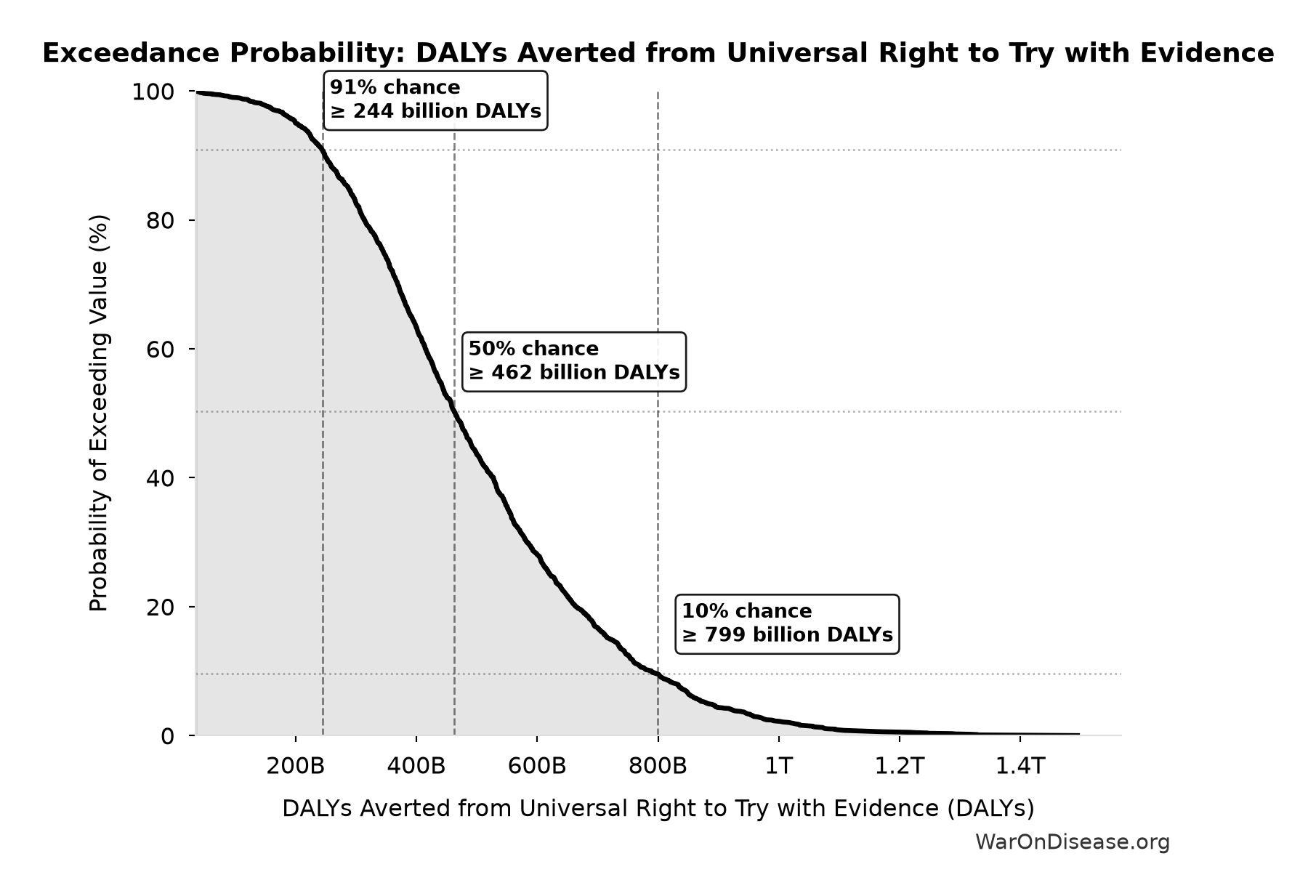
This exceedance probability chart shows the likelihood that DALYs Averted from Universal Right to Try with Evidence will exceed any given threshold. The higher the curve at a threshold, the more likely the value exceeds it.
Lives Saved from Universal Right to Try with Evidence: 9.19 billion deaths
Note📊 Details
Conditional cumulative premature deaths from global diseases and aging prevented across future generations by shifting the treatment-discovery schedule forward. The total can exceed the current population because it sums deaths prevented over the full acceleration period.
Inputs:
- Global Daily Deaths from Disease and Aging 📊: 150 thousand deaths/day (SE: ±7,500 deaths/day)
- Eventually Avoidable Death Percentage: 92.6% (95% CI: 50% - 98%)
- Average Treatment Acceleration from Universal Right to Try with Evidence 🔢: 181 years
\[ \begin{gathered} Lives_{RTT} \\ = Deaths_{disease,daily} \times Pct_{avoid,death} \times T_{accel,RTT} \times 365 \\ = 150{,}000 \times 92.6\% \times 181 \times 365 \\ = 9.19B \end{gathered} \] where: \[ \begin{gathered} T_{accel,RTT} \\ = T_{first,SQ} \times \left(1 - \frac{1}{k_{RTT}}\right) \\ = 222 \times \left(1 - \frac{1}{5.48}\right) \\ = 181 \end{gathered} \] where: \[ \begin{gathered} T_{first,SQ} \\ = T_{queue,SQ} \times 0.5 \\ = 443 \times 0.5 \\ = 222 \end{gathered} \] where: \[ \begin{gathered} T_{queue,SQ} \\ = \frac{N_{untreated}}{Treatments_{new,ann}} \\ = \frac{6{,}650}{15} \\ = 443 \end{gathered} \] where: \[ \begin{gathered} N_{untreated} \\ = N_{rare} \times 0.95 \\ = 7{,}000 \times 0.95 \\ = 6{,}650 \end{gathered} \] ? Low confidence
Sensitivity Analysis
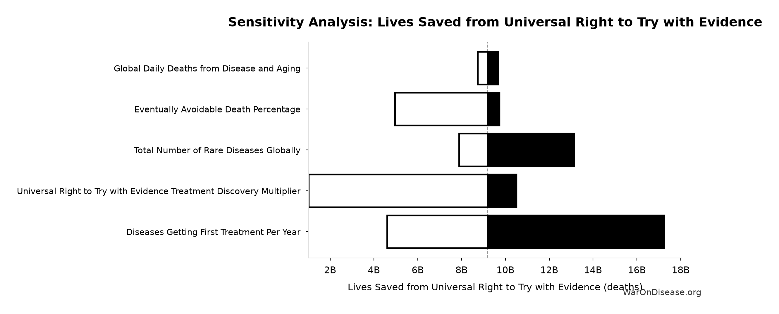
Sensitivity Indices for Lives Saved from Universal Right to Try with Evidence
Regression-based sensitivity showing which inputs explain the most variance in the output.
| Input Parameter | Sensitivity Coefficient | Interpretation |
|---|---|---|
| Average Treatment Acceleration from Universal Right to Try with Evidence (years) | 0.9436 | Strong driver |
| Eventually Avoidable Death Percentage (percentage) | 0.2710 | Weak driver |
| Global Daily Deaths from Disease and Aging (deaths/day) | 0.1115 | Weak driver |
Interpretation: Standardized coefficients show the change in output (in SD units) per 1 SD change in input. Values near ±1 indicate strong influence; values exceeding ±1 may occur with correlated inputs.
Monte Carlo Distribution
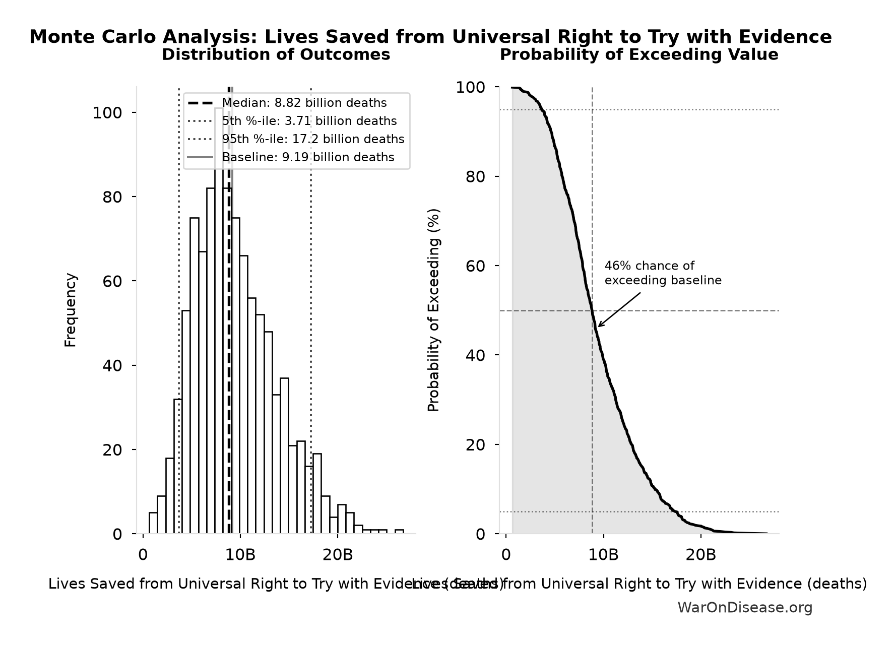
Simulation Results Summary: Lives Saved from Universal Right to Try with Evidence
| Statistic | Value |
|---|---|
| Baseline (deterministic) | 9.19 billion |
| Mean (expected value) | 9.4 billion |
| Median (50th percentile) | 8.82 billion |
| Standard Deviation | 4.13 billion |
| 90% Range (5th-95th percentile) | [3.71 billion, 17.2 billion] |
The histogram shows 1,000 of the 10,000 Monte Carlo draws for Lives Saved from Universal Right to Try with Evidence; the summary statistics use all 10,000. The exceedance curve (right) shows the probability of the outcome exceeding any given value.
Exceedance Probability
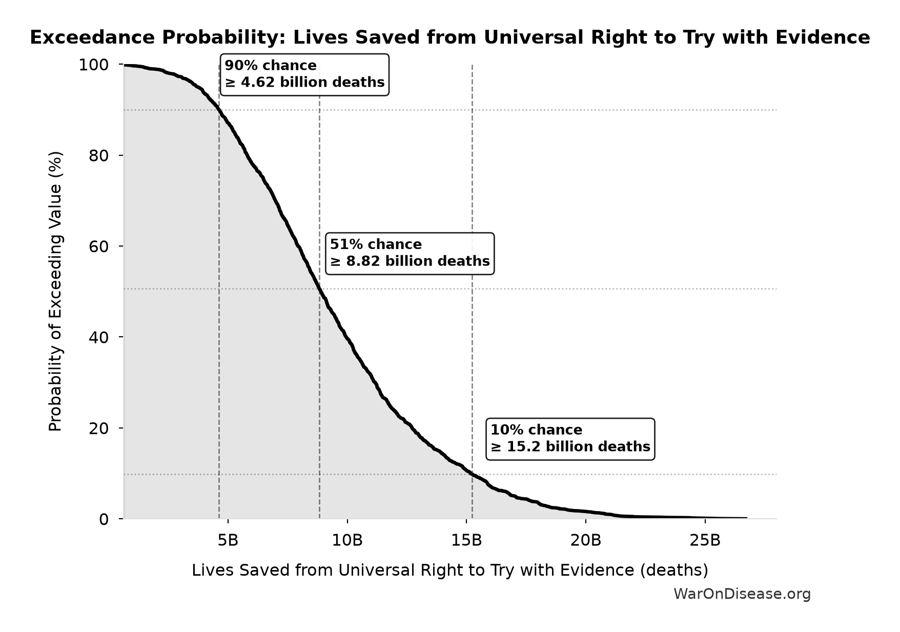
This exceedance probability chart shows the likelihood that Lives Saved from Universal Right to Try with Evidence will exceed any given threshold. The higher the curve at a threshold, the more likely the value exceeds it.
Disability-Equivalent Suffering Hours Prevented by Universal Right to Try with Evidence: 1.65 quadrillion hours
Note📊 Details
Conditional disability-equivalent hours prevented by the treatment schedule shift. Converts the years-lived-with-disability share of DALYs into hours; it does not claim every hour is an hour of conscious pain.
Inputs:
- DALYs Averted from Universal Right to Try with Evidence 🔢: 483 billion DALYs
- YLD Proportion of Total DALYs 📊: 0.39 proportion (SE: ±0.03 proportion)
\[ \begin{gathered} Hours_{suffer,RTT} \\ = DALYs_{RTT} \times Pct_{YLD} \times 8760 \\ = 483B \times 0.39 \times 8760 \\ = 1650T \end{gathered} \] where: \[ \begin{gathered} DALYs_{RTT} \\ = DALYs_{global,ann} \times Pct_{avoid,DALY} \times T_{accel,RTT} \\ = 2.88B \times 92.6\% \times 181 \\ = 483B \end{gathered} \] where: \[ \begin{gathered} T_{accel,RTT} \\ = T_{first,SQ} \times \left(1 - \frac{1}{k_{RTT}}\right) \\ = 222 \times \left(1 - \frac{1}{5.48}\right) \\ = 181 \end{gathered} \] where: \[ \begin{gathered} T_{first,SQ} \\ = T_{queue,SQ} \times 0.5 \\ = 443 \times 0.5 \\ = 222 \end{gathered} \] where: \[ \begin{gathered} T_{queue,SQ} \\ = \frac{N_{untreated}}{Treatments_{new,ann}} \\ = \frac{6{,}650}{15} \\ = 443 \end{gathered} \] where: \[ \begin{gathered} N_{untreated} \\ = N_{rare} \times 0.95 \\ = 7{,}000 \times 0.95 \\ = 6{,}650 \end{gathered} \] ? Low confidence
Sensitivity Analysis
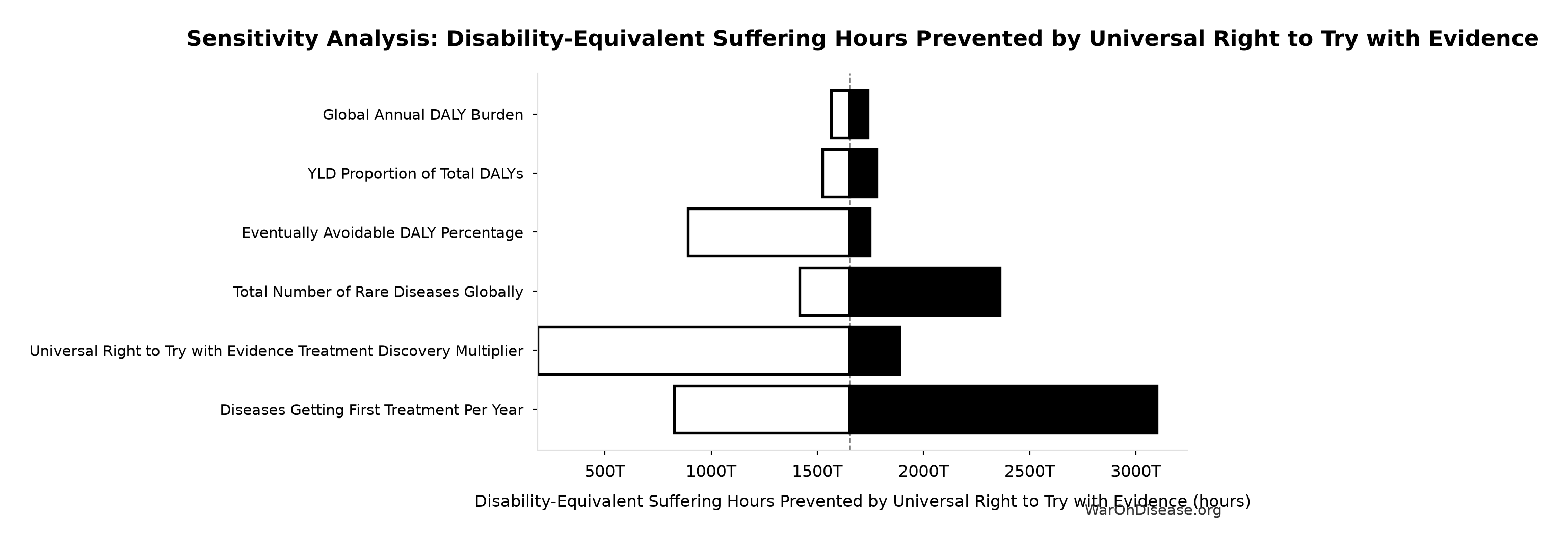
Sensitivity Indices for Disability-Equivalent Suffering Hours Prevented by Universal Right to Try with Evidence
Regression-based sensitivity showing which inputs explain the most variance in the output.
| Input Parameter | Sensitivity Coefficient | Interpretation |
|---|---|---|
| DALYs Averted from Universal Right to Try with Evidence (DALYs) | 0.9822 | Strong driver |
| YLD Proportion of Total DALYs (proportion) | 0.1721 | Weak driver |
Interpretation: Standardized coefficients show the change in output (in SD units) per 1 SD change in input. Values near ±1 indicate strong influence; values exceeding ±1 may occur with correlated inputs.
Monte Carlo Distribution
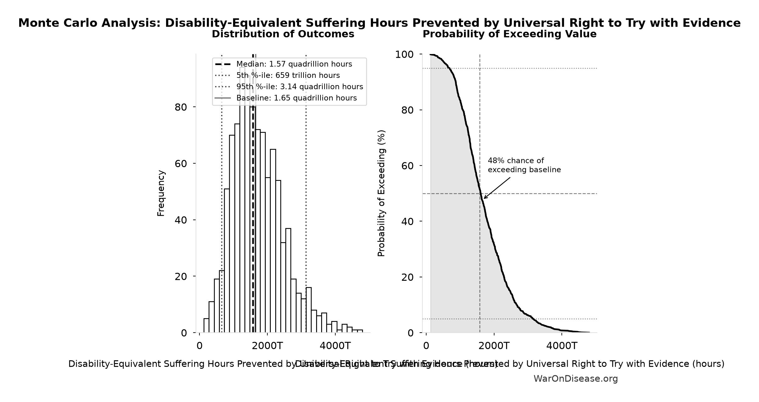
Simulation Results Summary: Disability-Equivalent Suffering Hours Prevented by Universal Right to Try with Evidence
| Statistic | Value |
|---|---|
| Baseline (deterministic) | 1.65 quadrillion |
| Mean (expected value) | 1.69 quadrillion |
| Median (50th percentile) | 1.57 quadrillion |
| Standard Deviation | 756 trillion |
| 90% Range (5th-95th percentile) | [659 trillion, 3.14 quadrillion] |
The histogram shows 1,000 of the 10,000 Monte Carlo draws for Disability-Equivalent Suffering Hours Prevented by Universal Right to Try with Evidence; the summary statistics use all 10,000. The exceedance curve (right) shows the probability of the outcome exceeding any given value.
Exceedance Probability
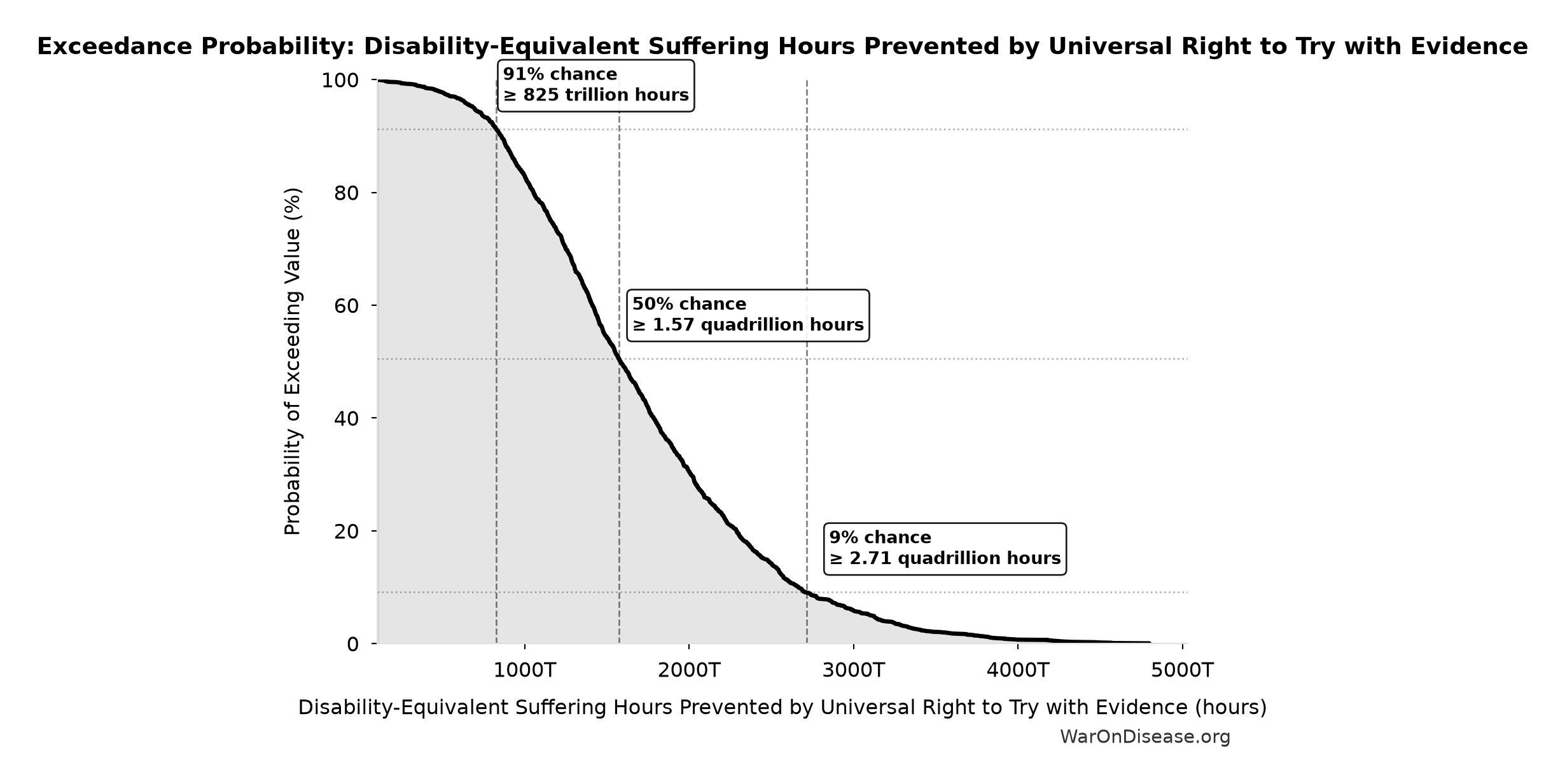
This exceedance probability chart shows the likelihood that Disability-Equivalent Suffering Hours Prevented by Universal Right to Try with Evidence will exceed any given threshold. The higher the curve at a threshold, the more likely the value exceeds it.
Disability-Equivalent Suffering Years Prevented by Universal Right to Try with Evidence: 189 billion years
Note📊 Details
Conditional disability-equivalent years of suffering prevented by the treatment schedule shift: the years-lived-with-disability share of the DALYs averted. A disability weight of 0.25 sustained for four years equals one full-disability-equivalent year; it does not claim every year is a year of maximum conscious pain.
Inputs:
- DALYs Averted from Universal Right to Try with Evidence 🔢: 483 billion DALYs
- YLD Proportion of Total DALYs 📊: 0.39 proportion (SE: ±0.03 proportion)
\[ \begin{gathered} Years_{suffer,RTT} \\ = DALYs_{RTT} \times Pct_{YLD} \\ = 483B \times 0.39 \\ = 189B \end{gathered} \] where: \[ \begin{gathered} DALYs_{RTT} \\ = DALYs_{global,ann} \times Pct_{avoid,DALY} \times T_{accel,RTT} \\ = 2.88B \times 92.6\% \times 181 \\ = 483B \end{gathered} \] where: \[ \begin{gathered} T_{accel,RTT} \\ = T_{first,SQ} \times \left(1 - \frac{1}{k_{RTT}}\right) \\ = 222 \times \left(1 - \frac{1}{5.48}\right) \\ = 181 \end{gathered} \] where: \[ \begin{gathered} T_{first,SQ} \\ = T_{queue,SQ} \times 0.5 \\ = 443 \times 0.5 \\ = 222 \end{gathered} \] where: \[ \begin{gathered} T_{queue,SQ} \\ = \frac{N_{untreated}}{Treatments_{new,ann}} \\ = \frac{6{,}650}{15} \\ = 443 \end{gathered} \] where: \[ \begin{gathered} N_{untreated} \\ = N_{rare} \times 0.95 \\ = 7{,}000 \times 0.95 \\ = 6{,}650 \end{gathered} \] ? Low confidence
Sensitivity Analysis
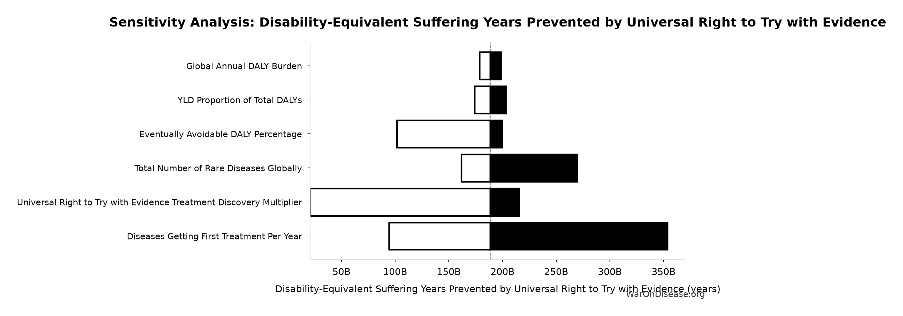
Sensitivity Indices for Disability-Equivalent Suffering Years Prevented by Universal Right to Try with Evidence
Regression-based sensitivity showing which inputs explain the most variance in the output.
| Input Parameter | Sensitivity Coefficient | Interpretation |
|---|---|---|
| DALYs Averted from Universal Right to Try with Evidence (DALYs) | 0.9822 | Strong driver |
| YLD Proportion of Total DALYs (proportion) | 0.1721 | Weak driver |
Interpretation: Standardized coefficients show the change in output (in SD units) per 1 SD change in input. Values near ±1 indicate strong influence; values exceeding ±1 may occur with correlated inputs.
Monte Carlo Distribution
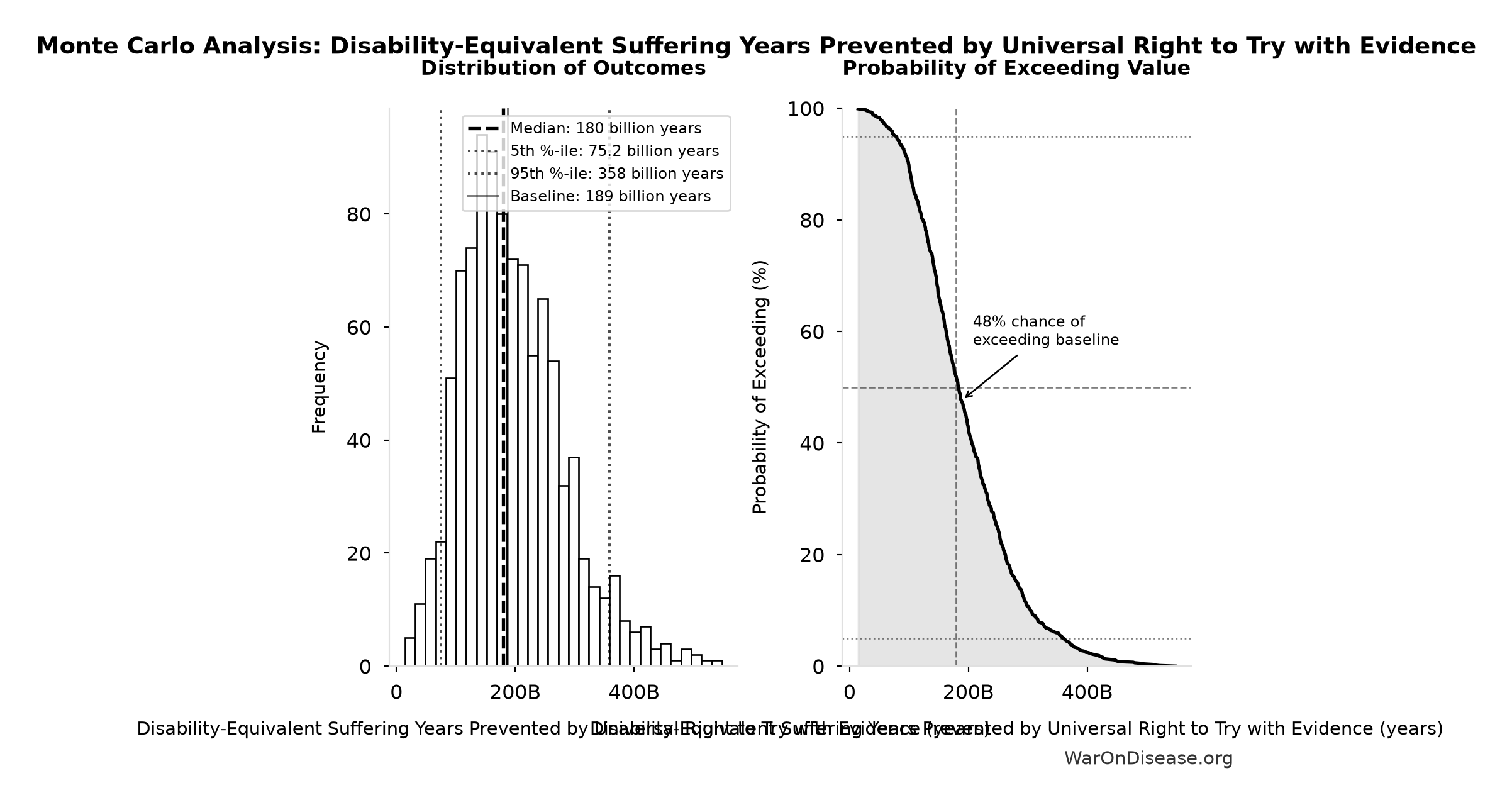
Simulation Results Summary: Disability-Equivalent Suffering Years Prevented by Universal Right to Try with Evidence
| Statistic | Value |
|---|---|
| Baseline (deterministic) | 189 billion |
| Mean (expected value) | 193 billion |
| Median (50th percentile) | 180 billion |
| Standard Deviation | 86.3 billion |
| 90% Range (5th-95th percentile) | [75.2 billion, 358 billion] |
The histogram shows 1,000 of the 10,000 Monte Carlo draws for Disability-Equivalent Suffering Years Prevented by Universal Right to Try with Evidence; the summary statistics use all 10,000. The exceedance curve (right) shows the probability of the outcome exceeding any given value.
Exceedance Probability
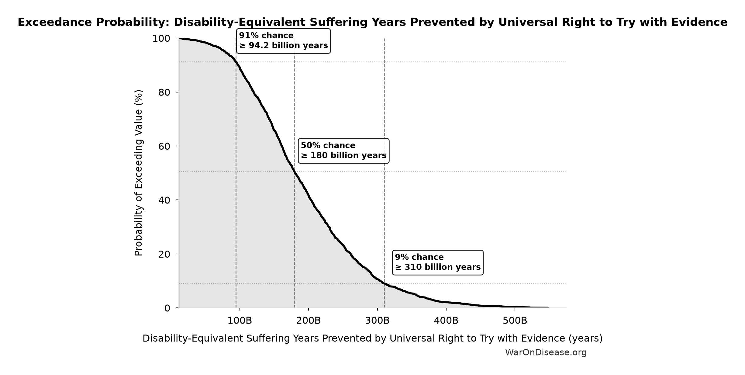
This exceedance probability chart shows the likelihood that Disability-Equivalent Suffering Years Prevented by Universal Right to Try with Evidence will exceed any given threshold. The higher the curve at a threshold, the more likely the value exceeds it.
Average Treatment Acceleration from Universal Right to Try with Evidence: 181 years
Note📊 Details
Average years earlier the first effective treatment arrives across the global therapeutic frontier after all 50 states adopt Universal Right to Try with Evidence. Uses the same schedule-shift structure as the 1% Treaty impact model: the status quo discovery timeline multiplied by one minus the inverse treatment-discovery multiplier.
Inputs:
- Status Quo Average Years to First Treatment 🔢: 222 years
- Universal Right to Try with Evidence Treatment Discovery Multiplier: 5.48x (95% CI: 1.1x - 15x)
\[ \begin{gathered} T_{accel,RTT} \\ = T_{first,SQ} \times \left(1 - \frac{1}{k_{RTT}}\right) \\ = 222 \times \left(1 - \frac{1}{5.48}\right) \\ = 181 \end{gathered} \] where: \[ \begin{gathered} T_{first,SQ} \\ = T_{queue,SQ} \times 0.5 \\ = 443 \times 0.5 \\ = 222 \end{gathered} \] where: \[ \begin{gathered} T_{queue,SQ} \\ = \frac{N_{untreated}}{Treatments_{new,ann}} \\ = \frac{6{,}650}{15} \\ = 443 \end{gathered} \] where: \[ \begin{gathered} N_{untreated} \\ = N_{rare} \times 0.95 \\ = 7{,}000 \times 0.95 \\ = 6{,}650 \end{gathered} \] ? Low confidence
Sensitivity Analysis
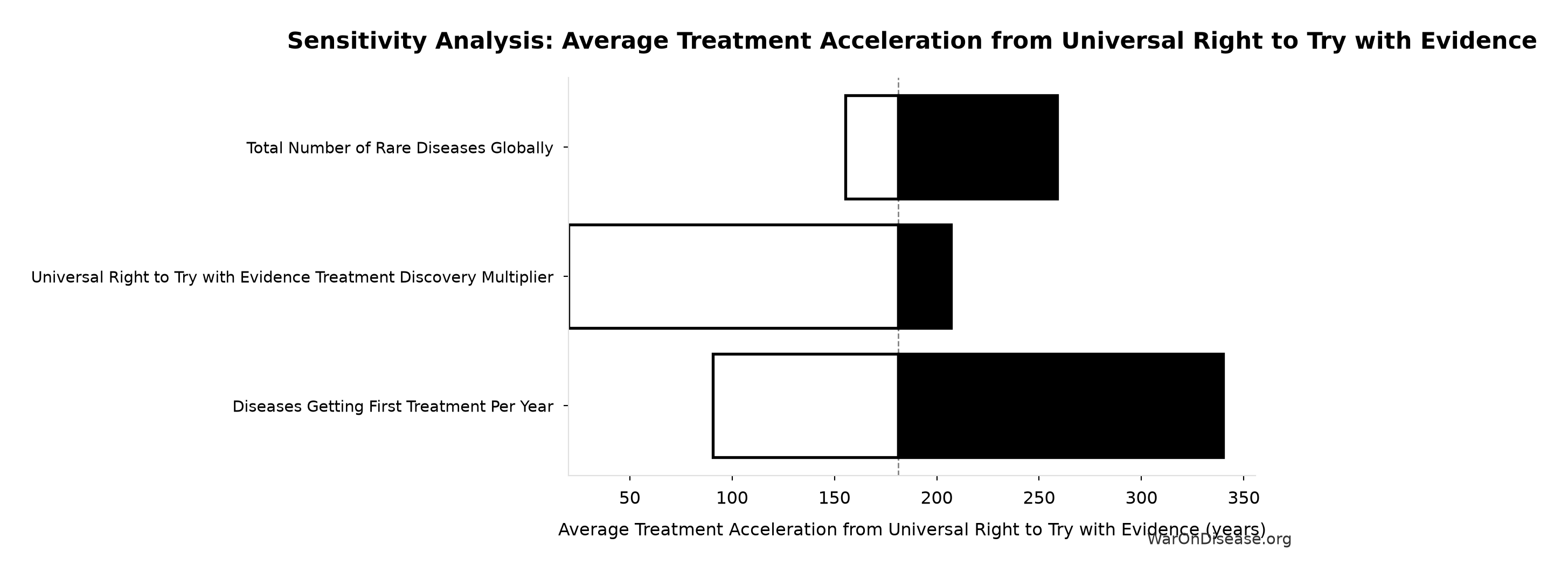
Sensitivity Indices for Average Treatment Acceleration from Universal Right to Try with Evidence
Regression-based sensitivity showing which inputs explain the most variance in the output.
| Input Parameter | Sensitivity Coefficient | Interpretation |
|---|---|---|
| Status Quo Average Years to First Treatment (years) | 0.8444 | Strong driver |
| Universal Right to Try with Evidence Treatment Discovery Multiplier (x) | 0.3959 | Moderate driver |
Interpretation: Standardized coefficients show the change in output (in SD units) per 1 SD change in input. Values near ±1 indicate strong influence; values exceeding ±1 may occur with correlated inputs.
Monte Carlo Distribution
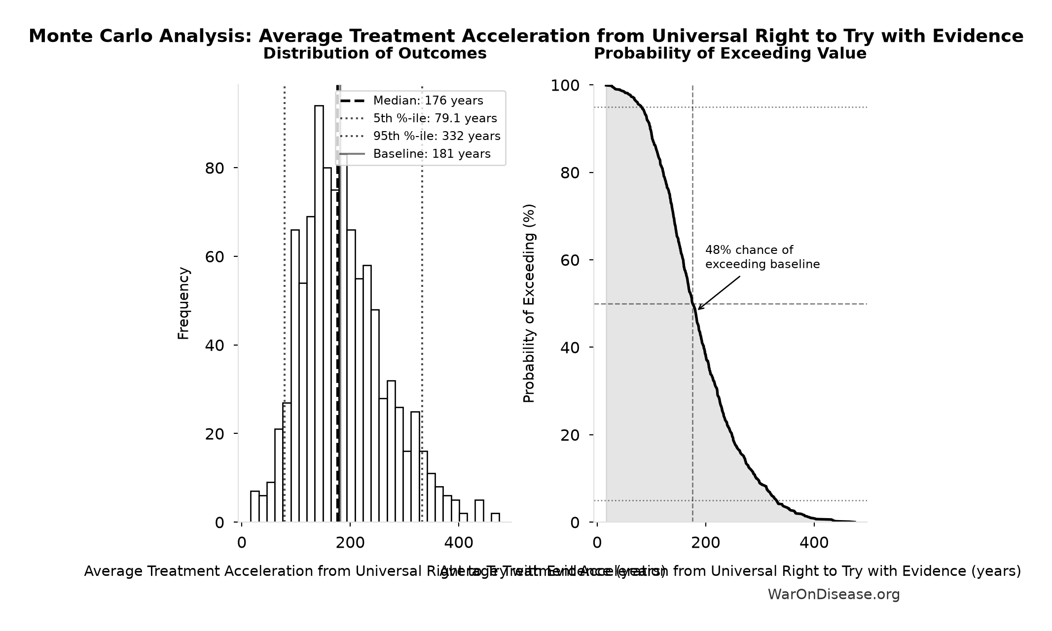
Simulation Results Summary: Average Treatment Acceleration from Universal Right to Try with Evidence
| Statistic | Value |
|---|---|
| Baseline (deterministic) | 181 |
| Mean (expected value) | 187 |
| Median (50th percentile) | 176 |
| Standard Deviation | 77.8 |
| 90% Range (5th-95th percentile) | [79.1, 332] |
The histogram shows 1,000 of the 10,000 Monte Carlo draws for Average Treatment Acceleration from Universal Right to Try with Evidence; the summary statistics use all 10,000. The exceedance curve (right) shows the probability of the outcome exceeding any given value.
Exceedance Probability
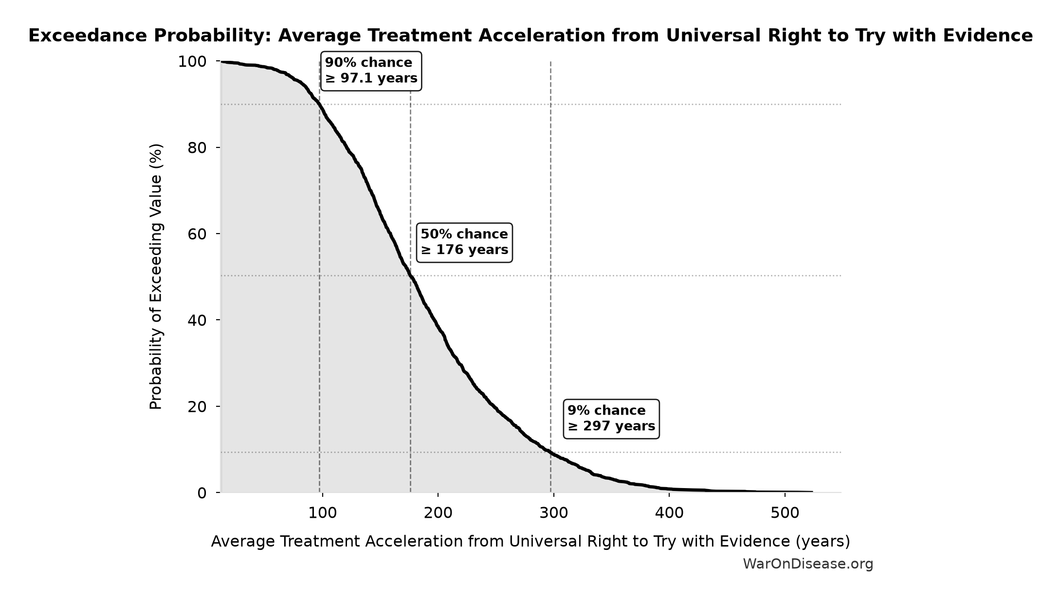
This exceedance probability chart shows the likelihood that Average Treatment Acceleration from Universal Right to Try with Evidence will exceed any given threshold. The higher the curve at a threshold, the more likely the value exceeds it.
Universal Right to Try with Evidence Cost-Effectiveness vs GiveWell Range Midpoint: 636.2kx
Note📊 Details
Conditional cost-effectiveness of adopting Universal Right to Try with Evidence in all 50 states relative to the midpoint of GiveWell’s cited modeled cost-per-life-saved range. The cost scopes differ: the Right to Try numerator counts only the campaign and registry launch and excludes patient and payer spending on treatment delivery, trial-site services, and permitted study costs, while the GiveWell figure includes full program costs. This comparison is valid only if full adoption and mature implementation produce the modeled treatment schedule shift.
Inputs:
- GiveWell Midpoint of Modeled Cost per Life Saved Range 📊: $4,500
- Universal Right to Try with Evidence Implementation Cost per Life Saved 🔢: $0.00707
\[ \begin{gathered} k_{RTT,GiveWell} \\ = \frac{Cost_{GW,avg}}{Cost_{RTT,life}} \\ = \frac{\$4.5K}{\$0.00707} \\ = 636{,}000 \end{gathered} \] where: \[ \begin{gathered} Cost_{RTT,life} \\ = \frac{C_{RTT}}{Lives_{RTT}} \\ = \frac{\$65M}{9.19B} \\ = \$0.00707 \end{gathered} \] where: \[ \begin{gathered} Lives_{RTT} \\ = Deaths_{disease,daily} \times Pct_{avoid,death} \times T_{accel,RTT} \times 365 \\ = 150{,}000 \times 92.6\% \times 181 \times 365 \\ = 9.19B \end{gathered} \] where: \[ \begin{gathered} T_{accel,RTT} \\ = T_{first,SQ} \times \left(1 - \frac{1}{k_{RTT}}\right) \\ = 222 \times \left(1 - \frac{1}{5.48}\right) \\ = 181 \end{gathered} \] where: \[ \begin{gathered} T_{first,SQ} \\ = T_{queue,SQ} \times 0.5 \\ = 443 \times 0.5 \\ = 222 \end{gathered} \] where: \[ \begin{gathered} T_{queue,SQ} \\ = \frac{N_{untreated}}{Treatments_{new,ann}} \\ = \frac{6{,}650}{15} \\ = 443 \end{gathered} \] where: \[ \begin{gathered} N_{untreated} \\ = N_{rare} \times 0.95 \\ = 7{,}000 \times 0.95 \\ = 6{,}650 \end{gathered} \] ? Low confidence
Sensitivity Analysis
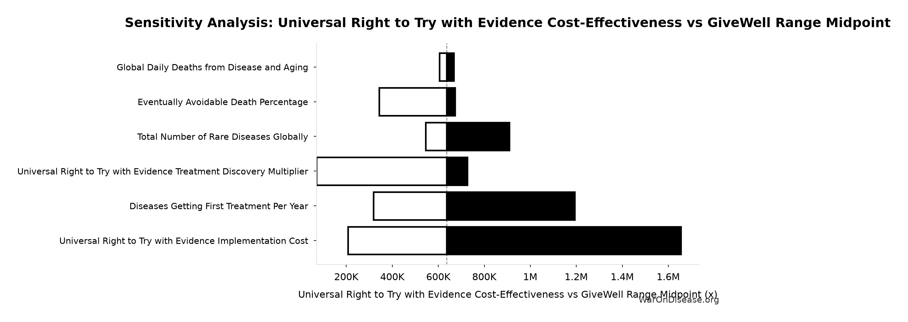
Sensitivity Indices for Universal Right to Try with Evidence Cost-Effectiveness vs GiveWell Range Midpoint
Regression-based sensitivity showing which inputs explain the most variance in the output.
| Input Parameter | Sensitivity Coefficient | Interpretation |
|---|---|---|
| Universal Right to Try with Evidence Implementation Cost per Life Saved (USD/life) | -0.5475 | Strong driver |
Interpretation: Standardized coefficients show the change in output (in SD units) per 1 SD change in input. Values near ±1 indicate strong influence; values exceeding ±1 may occur with correlated inputs.
Monte Carlo Distribution
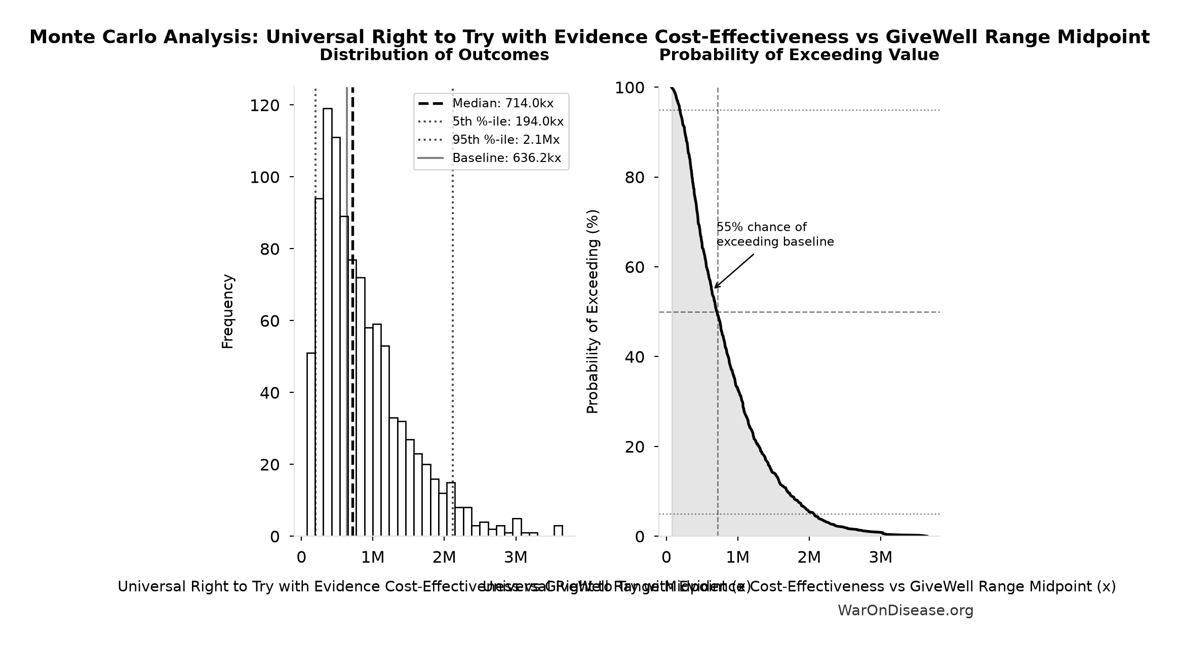
Simulation Results Summary: Universal Right to Try with Evidence Cost-Effectiveness vs GiveWell Range Midpoint
| Statistic | Value |
|---|---|
| Baseline (deterministic) | 636.2kx |
| Mean (expected value) | 873.8kx |
| Median (50th percentile) | 714.0kx |
| Standard Deviation | 619.3kx |
| 90% Range (5th-95th percentile) | [194.0kx, 2.1Mx] |
The histogram shows 1,000 of the 10,000 Monte Carlo draws for Universal Right to Try with Evidence Cost-Effectiveness vs GiveWell Range Midpoint; the summary statistics use all 10,000. The exceedance curve (right) shows the probability of the outcome exceeding any given value.
Exceedance Probability
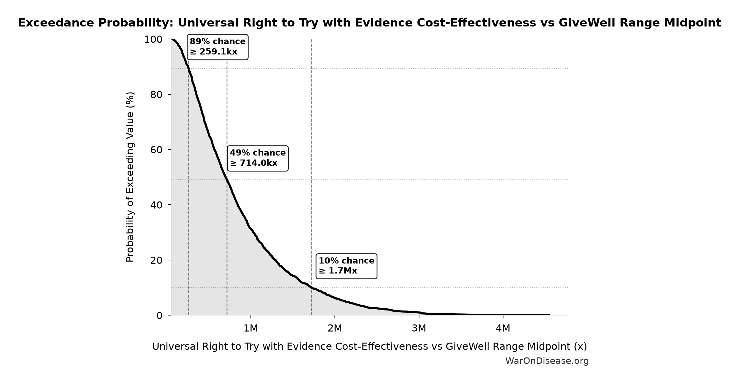
This exceedance probability chart shows the likelihood that Universal Right to Try with Evidence Cost-Effectiveness vs GiveWell Range Midpoint will exceed any given threshold. The higher the curve at a threshold, the more likely the value exceeds it.
Status Quo Average Years to First Treatment: 222 years
Note📊 Details
Average years until first treatment discovered for a typical disease under current system. At current discovery rates, the average disease waits half the total exploration time (~443/2 = ~222 years).
Inputs:
- Status Quo Therapeutic Space Exploration Time 🔢: 443 years
\[ \begin{gathered} T_{first,SQ} \\ = T_{queue,SQ} \times 0.5 \\ = 443 \times 0.5 \\ = 222 \end{gathered} \] where: \[ \begin{gathered} T_{queue,SQ} \\ = \frac{N_{untreated}}{Treatments_{new,ann}} \\ = \frac{6{,}650}{15} \\ = 443 \end{gathered} \] where: \[ \begin{gathered} N_{untreated} \\ = N_{rare} \times 0.95 \\ = 7{,}000 \times 0.95 \\ = 6{,}650 \end{gathered} \] Methodology:38
? Low confidence
Sensitivity Analysis
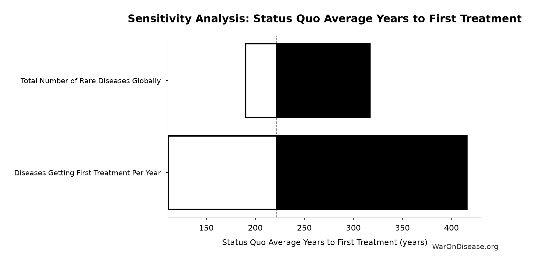
Sensitivity Indices for Status Quo Average Years to First Treatment
Regression-based sensitivity showing which inputs explain the most variance in the output.
| Input Parameter | Sensitivity Coefficient | Interpretation |
|---|---|---|
| Status Quo Therapeutic Space Exploration Time (years) | 1.0000 | Strong driver |
Interpretation: Standardized coefficients show the change in output (in SD units) per 1 SD change in input. Values near ±1 indicate strong influence; values exceeding ±1 may occur with correlated inputs.
Monte Carlo Distribution
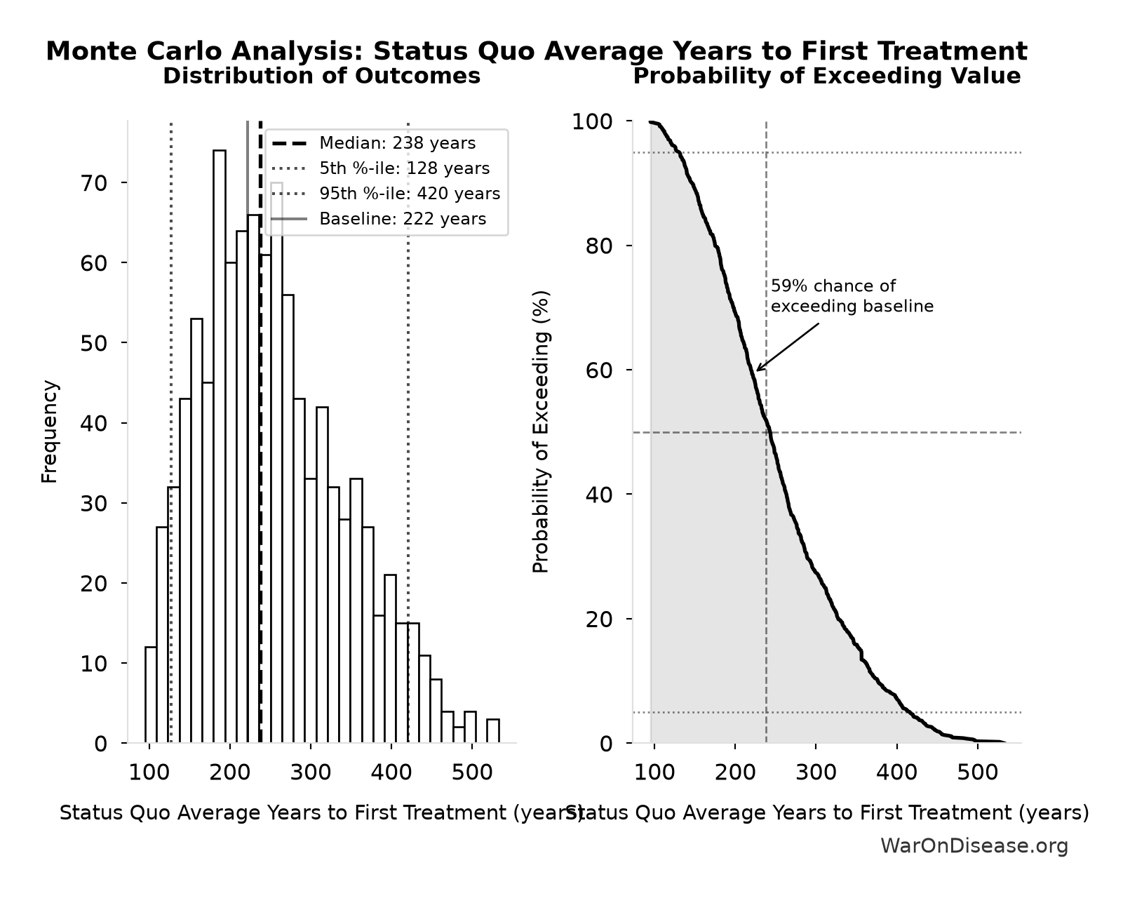
Simulation Results Summary: Status Quo Average Years to First Treatment
| Statistic | Value |
|---|---|
| Baseline (deterministic) | 222 |
| Mean (expected value) | 251 |
| Median (50th percentile) | 238 |
| Standard Deviation | 88.8 |
| 90% Range (5th-95th percentile) | [128, 420] |
The histogram shows 1,000 of the 10,000 Monte Carlo draws for Status Quo Average Years to First Treatment; the summary statistics use all 10,000. The exceedance curve (right) shows the probability of the outcome exceeding any given value.
Exceedance Probability
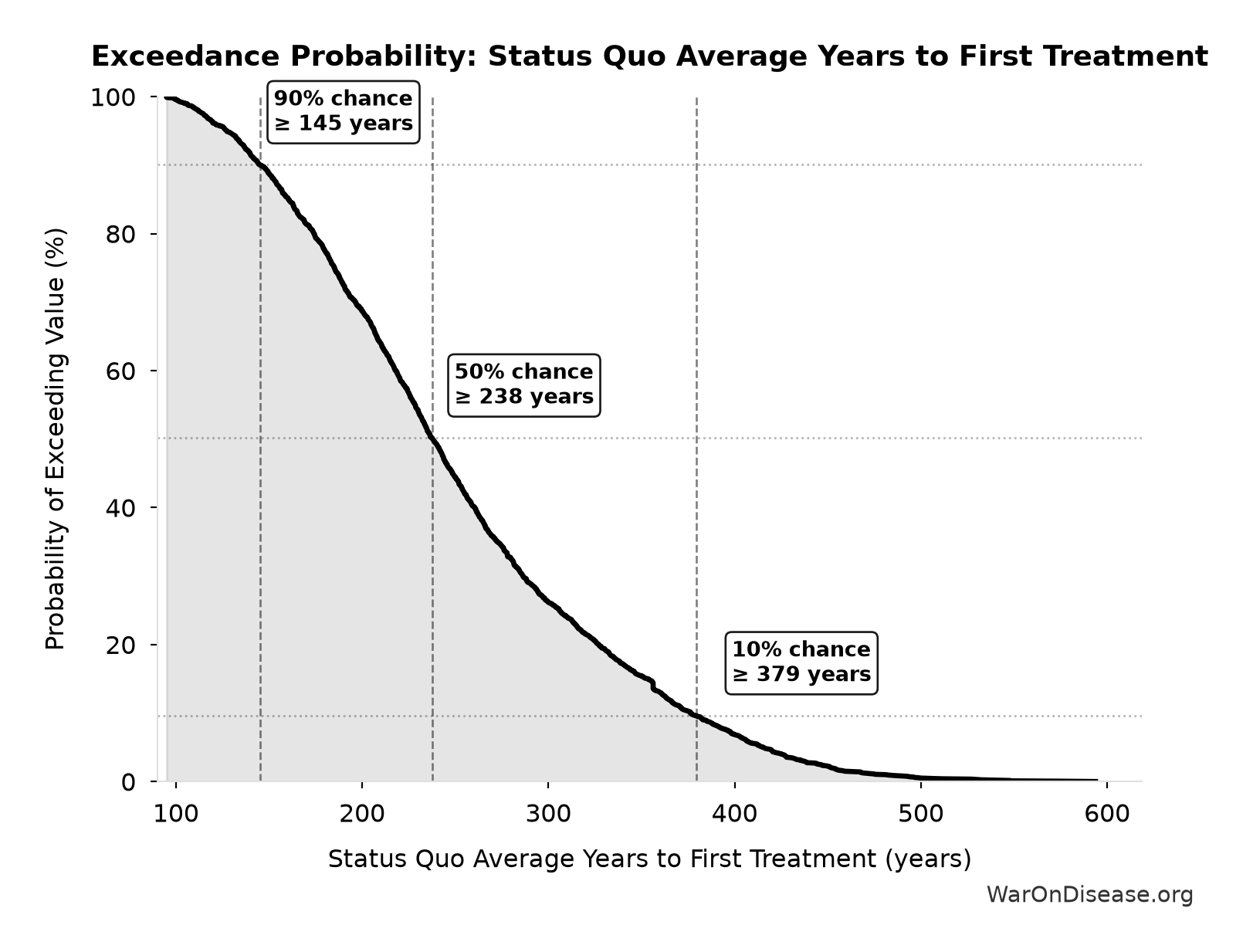
This exceedance probability chart shows the likelihood that Status Quo Average Years to First Treatment will exceed any given threshold. The higher the curve at a threshold, the more likely the value exceeds it.
Status Quo Therapeutic Space Exploration Time: 443 years
Note📊 Details
Years to explore the entire therapeutic search space under current system. At current discovery rate of ~15 diseases/year getting first treatments, finding treatments for all ~6,650 untreated diseases would take ~443 years.
Inputs:
- Diseases Without Effective Treatment 🔢: 6,650 diseases
- Diseases Getting First Treatment Per Year 📊: 15 diseases/year (95% CI: 8 diseases/year - 30 diseases/year)
\[ \begin{gathered} T_{queue,SQ} \\ = \frac{N_{untreated}}{Treatments_{new,ann}} \\ = \frac{6{,}650}{15} \\ = 443 \end{gathered} \] where: \[ \begin{gathered} N_{untreated} \\ = N_{rare} \times 0.95 \\ = 7{,}000 \times 0.95 \\ = 6{,}650 \end{gathered} \] Methodology:38
? Low confidence
Sensitivity Analysis
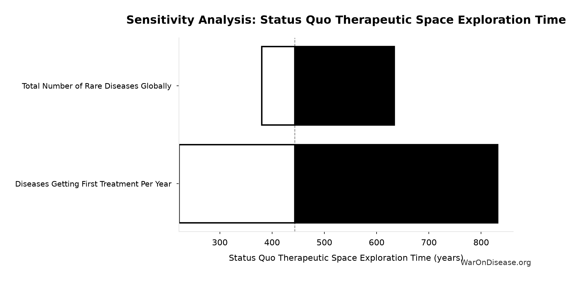
Sensitivity Indices for Status Quo Therapeutic Space Exploration Time
Regression-based sensitivity showing which inputs explain the most variance in the output.
| Input Parameter | Sensitivity Coefficient | Interpretation |
|---|---|---|
| Diseases Getting First Treatment Per Year (diseases/year) | -0.8696 | Strong driver |
| Diseases Without Effective Treatment (diseases) | 0.3427 | Moderate driver |
Interpretation: Standardized coefficients show the change in output (in SD units) per 1 SD change in input. Values near ±1 indicate strong influence; values exceeding ±1 may occur with correlated inputs.
Monte Carlo Distribution
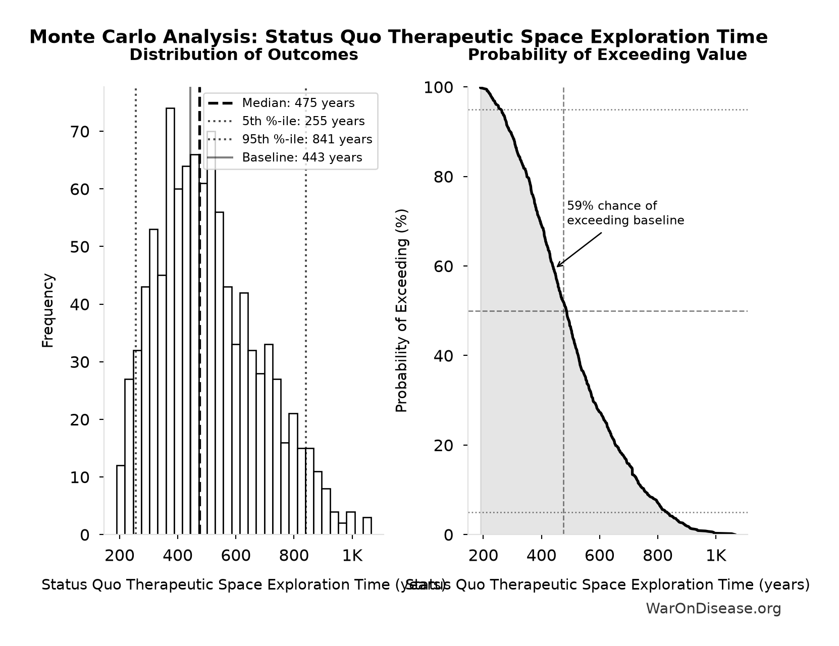
Simulation Results Summary: Status Quo Therapeutic Space Exploration Time
| Statistic | Value |
|---|---|
| Baseline (deterministic) | 443 |
| Mean (expected value) | 502 |
| Median (50th percentile) | 475 |
| Standard Deviation | 178 |
| 90% Range (5th-95th percentile) | [255, 841] |
The histogram shows 1,000 of the 10,000 Monte Carlo draws for Status Quo Therapeutic Space Exploration Time; the summary statistics use all 10,000. The exceedance curve (right) shows the probability of the outcome exceeding any given value.
Exceedance Probability
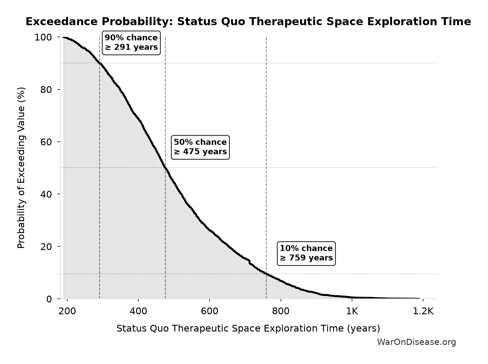
This exceedance probability chart shows the likelihood that Status Quo Therapeutic Space Exploration Time will exceed any given threshold. The higher the curve at a threshold, the more likely the value exceeds it.
Thalidomide DALYs Per Event: 41,760 DALYs
Note📊 Details
Total DALYs per US-scale thalidomide event (YLL + YLD)
Inputs:
- Thalidomide YLD Per Event 🔢: 12,960 years
- Thalidomide YLL Per Event 🔢: 28,800 years
\[ \begin{gathered} DALY_{thal} \\ = YLD_{thal} + YLL_{thal} \\ = 13{,}000 + 28{,}800 \\ = 41{,}800 \end{gathered} \] where: \[ \begin{gathered} YLD_{thal} \\ = DW_{thal} \times N_{thal,survive} \times LE_{thal} \\ = 0.4 \times 540 \times 60 \\ = 13{,}000 \end{gathered} \] where: \[ \begin{gathered} N_{thal,survive} \\ = N_{thal,US,prevent} \times (1 - Rate_{thal,mort}) \\ = 900 \times (1 - 40\%) \\ = 540 \end{gathered} \] where: \[ \begin{gathered} N_{thal,US,prevent} \\ = N_{thal,global} \times Pct_{US,1960} \\ = 15{,}000 \times 6\% \\ = 900 \end{gathered} \] where: \[ \begin{gathered} YLL_{thal} \\ = Deaths_{thal} \times 80 \\ = 360 \times 80 \\ = 28{,}800 \end{gathered} \] where: \[ \begin{gathered} Deaths_{thal} \\ = Rate_{thal,mort} \times N_{thal,US,prevent} \\ = 40\% \times 900 \\ = 360 \end{gathered} \] ~ Medium confidence
Sensitivity Analysis
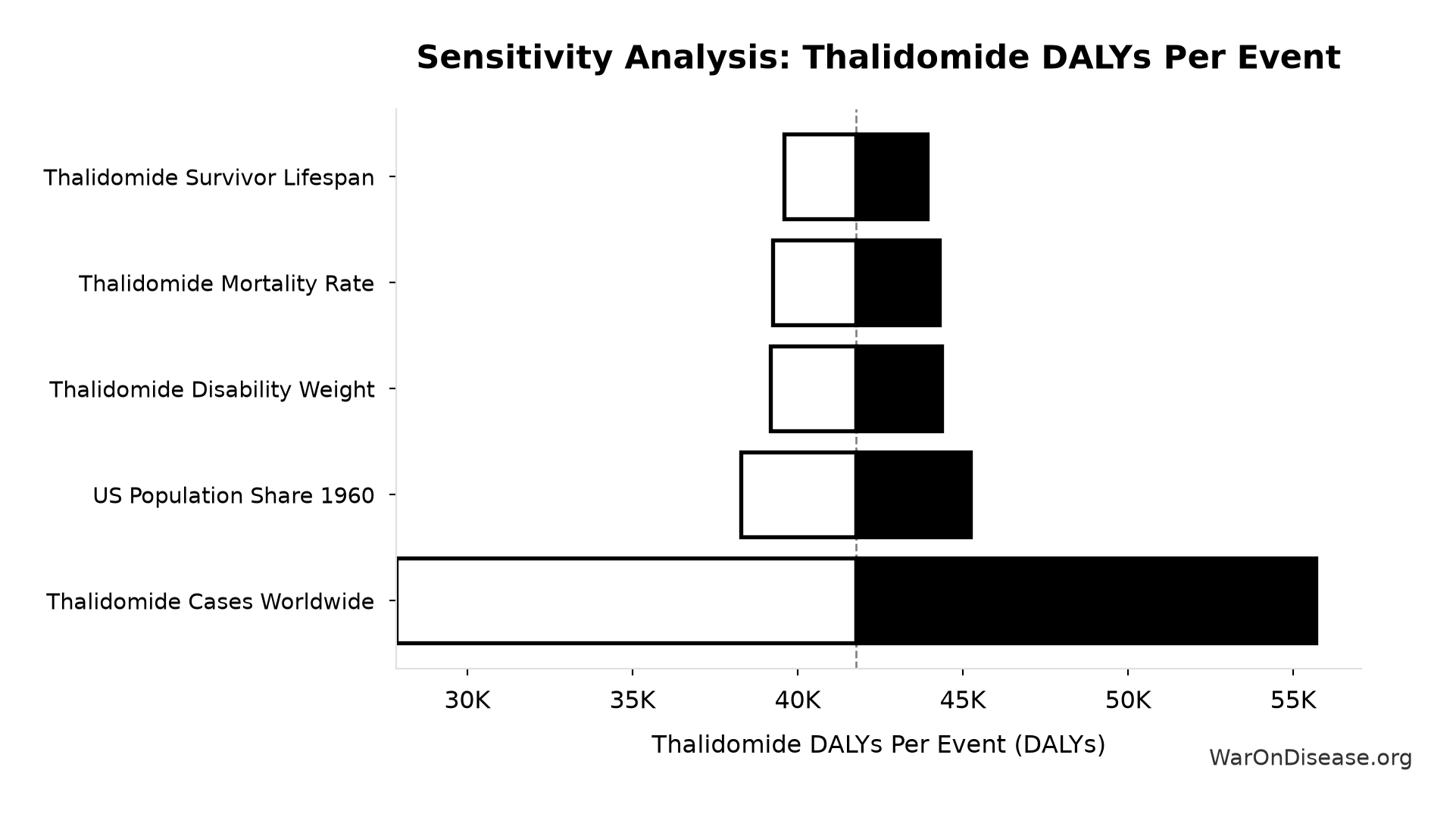
Sensitivity Indices for Thalidomide DALYs Per Event
Regression-based sensitivity showing which inputs explain the most variance in the output.
| Input Parameter | Sensitivity Coefficient | Interpretation |
|---|---|---|
| Thalidomide YLL Per Event (years) | 0.7035 | Strong driver |
| Thalidomide YLD Per Event (years) | 0.3838 | Moderate driver |
Interpretation: Standardized coefficients show the change in output (in SD units) per 1 SD change in input. Values near ±1 indicate strong influence; values exceeding ±1 may occur with correlated inputs.
Monte Carlo Distribution
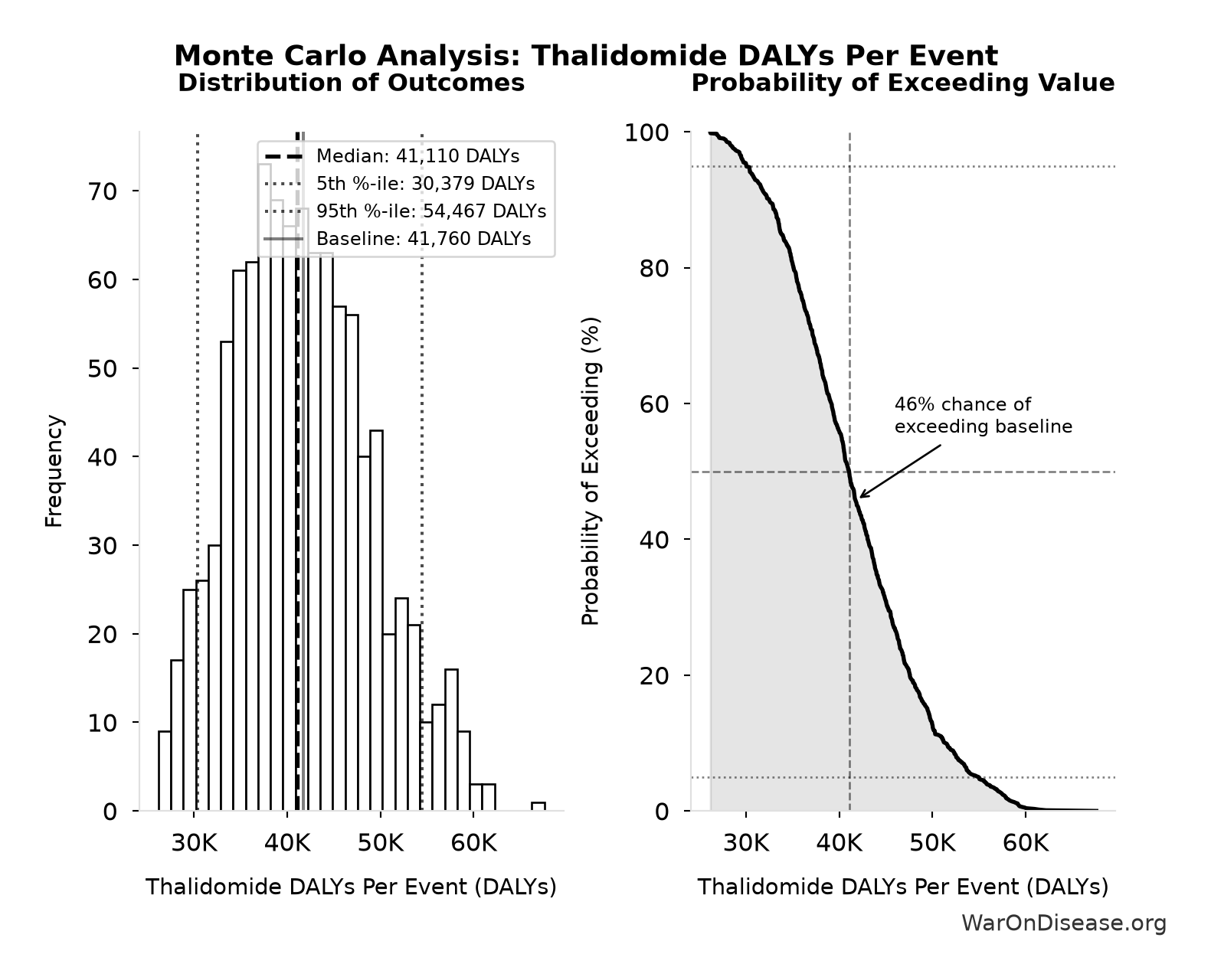
Simulation Results Summary: Thalidomide DALYs Per Event
| Statistic | Value |
|---|---|
| Baseline (deterministic) | 41,760 |
| Mean (expected value) | 41,590 |
| Median (50th percentile) | 41,110 |
| Standard Deviation | 7,233 |
| 90% Range (5th-95th percentile) | [30,379, 54,467] |
The histogram shows 1,000 of the 10,000 Monte Carlo draws for Thalidomide DALYs Per Event; the summary statistics use all 10,000. The exceedance curve (right) shows the probability of the outcome exceeding any given value.
Exceedance Probability
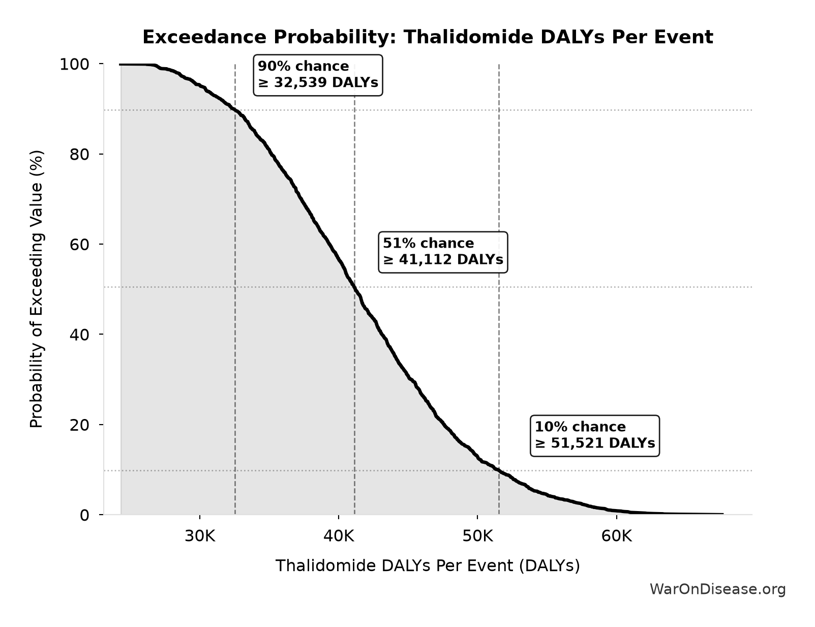
This exceedance probability chart shows the likelihood that Thalidomide DALYs Per Event will exceed any given threshold. The higher the curve at a threshold, the more likely the value exceeds it.
Thalidomide Deaths Per Event: 360 deaths
Note📊 Details
Deaths per US-scale thalidomide event
Inputs:
- Thalidomide Mortality Rate 📊: 40% (95% CI: 35% - 45%)
- Thalidomide US Cases Prevented 🔢: 900 cases
\[ \begin{gathered} Deaths_{thal} \\ = Rate_{thal,mort} \times N_{thal,US,prevent} \\ = 40\% \times 900 \\ = 360 \end{gathered} \] where: \[ \begin{gathered} N_{thal,US,prevent} \\ = N_{thal,global} \times Pct_{US,1960} \\ = 15{,}000 \times 6\% \\ = 900 \end{gathered} \] ~ Medium confidence
Sensitivity Analysis
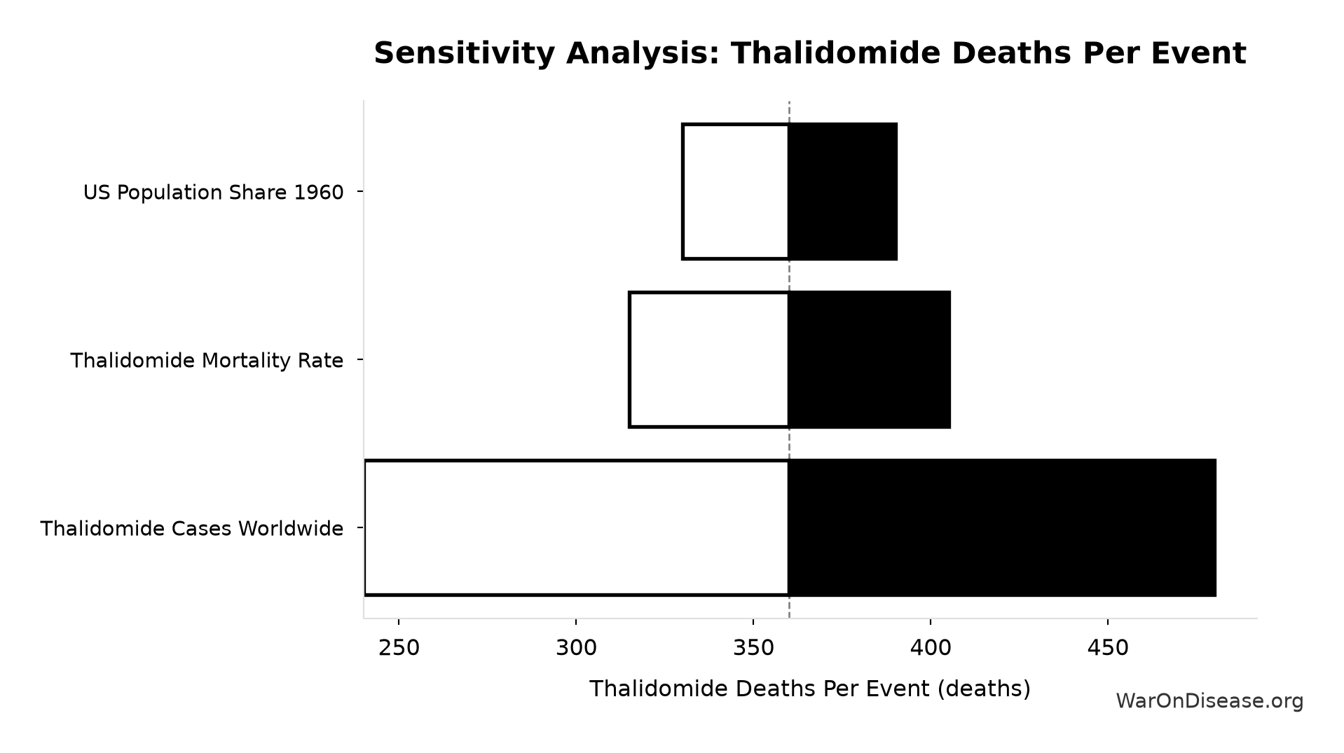
Sensitivity Indices for Thalidomide Deaths Per Event
Regression-based sensitivity showing which inputs explain the most variance in the output.
| Input Parameter | Sensitivity Coefficient | Interpretation |
|---|---|---|
| Thalidomide US Cases Prevented (cases) | 0.9385 | Strong driver |
| Thalidomide Mortality Rate (percentage) | 0.3437 | Moderate driver |
Interpretation: Standardized coefficients show the change in output (in SD units) per 1 SD change in input. Values near ±1 indicate strong influence; values exceeding ±1 may occur with correlated inputs.
Monte Carlo Distribution
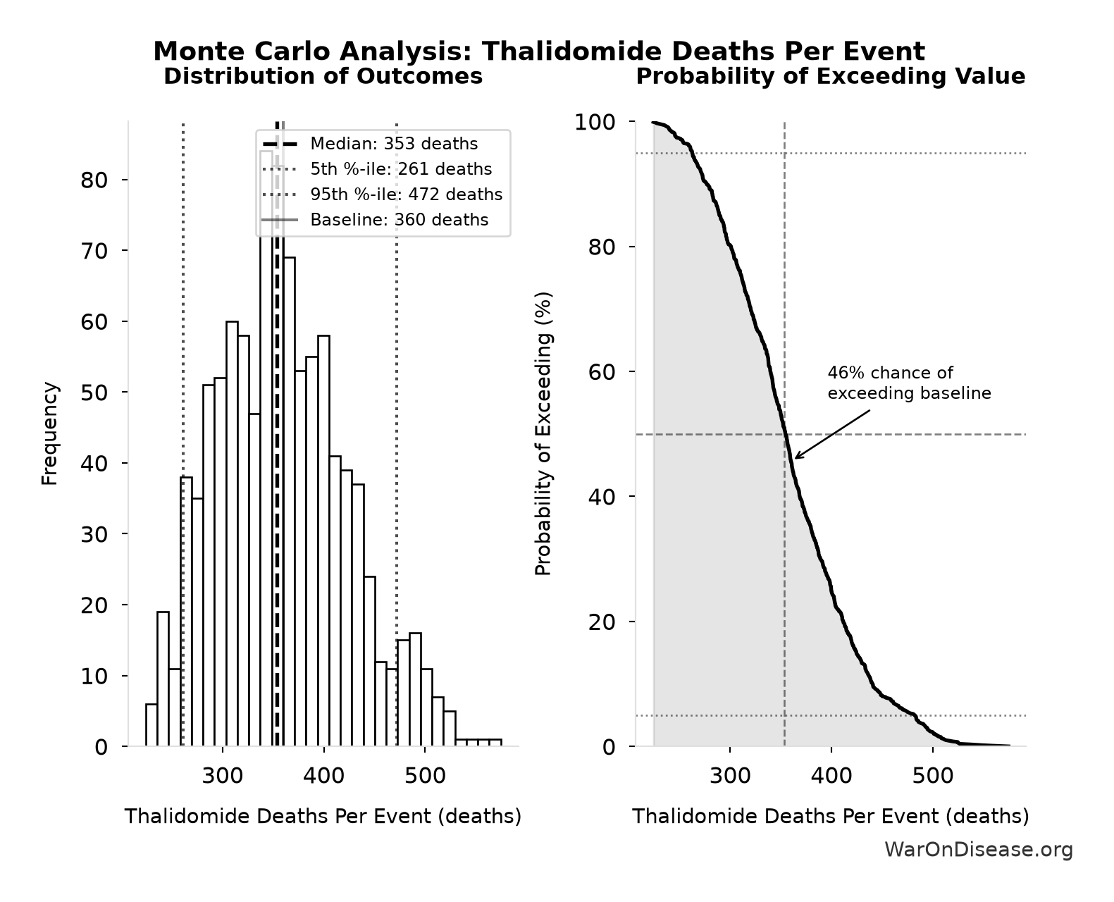
Simulation Results Summary: Thalidomide Deaths Per Event
| Statistic | Value |
|---|---|
| Baseline (deterministic) | 360 |
| Mean (expected value) | 359 |
| Median (50th percentile) | 353 |
| Standard Deviation | 63.6 |
| 90% Range (5th-95th percentile) | [261, 472] |
The histogram shows 1,000 of the 10,000 Monte Carlo draws for Thalidomide Deaths Per Event; the summary statistics use all 10,000. The exceedance curve (right) shows the probability of the outcome exceeding any given value.
Exceedance Probability
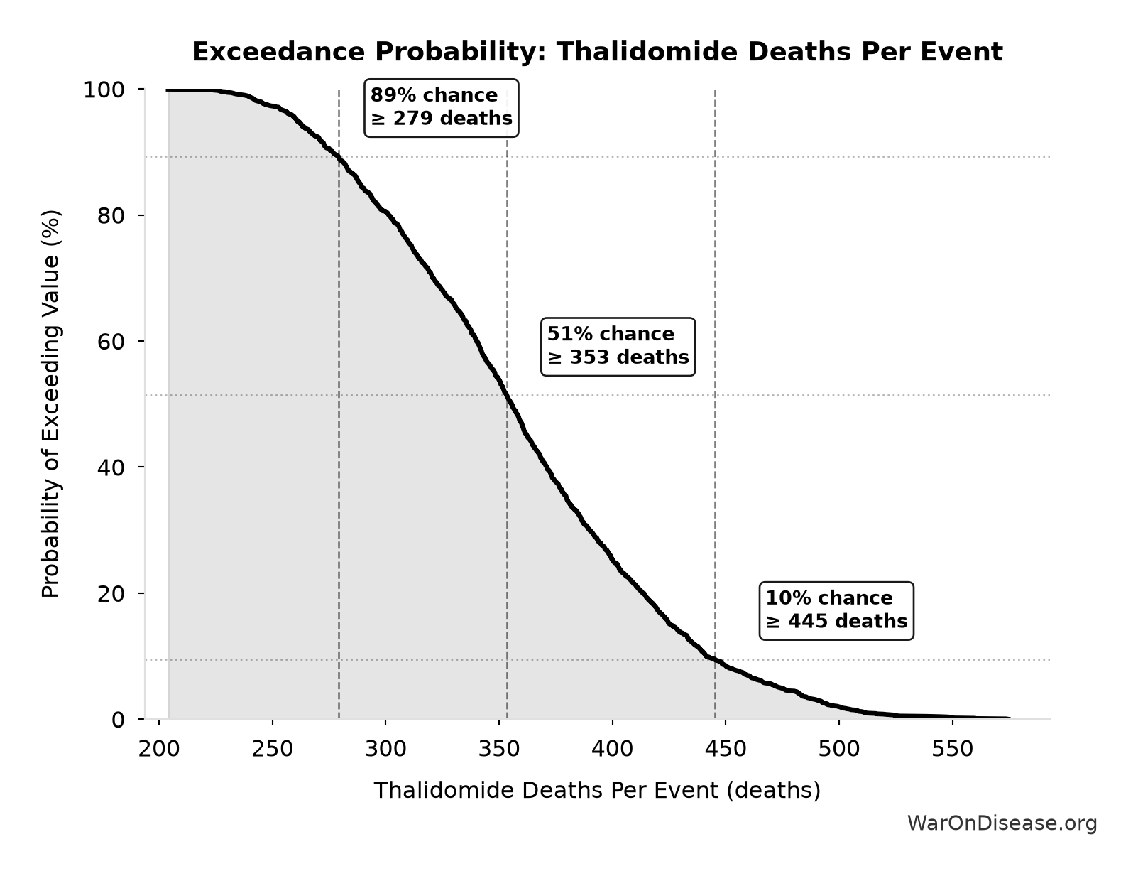
This exceedance probability chart shows the likelihood that Thalidomide Deaths Per Event will exceed any given threshold. The higher the curve at a threshold, the more likely the value exceeds it.
Thalidomide Survivors Per Event: 540 cases
Note📊 Details
Survivors per US-scale thalidomide event
Inputs:
- Thalidomide Mortality Rate 📊: 40% (95% CI: 35% - 45%)
- Thalidomide US Cases Prevented 🔢: 900 cases
\[ \begin{gathered} N_{thal,survive} \\ = N_{thal,US,prevent} \times (1 - Rate_{thal,mort}) \\ = 900 \times (1 - 40\%) \\ = 540 \end{gathered} \] where: \[ \begin{gathered} N_{thal,US,prevent} \\ = N_{thal,global} \times Pct_{US,1960} \\ = 15{,}000 \times 6\% \\ = 900 \end{gathered} \] ~ Medium confidence
Sensitivity Analysis
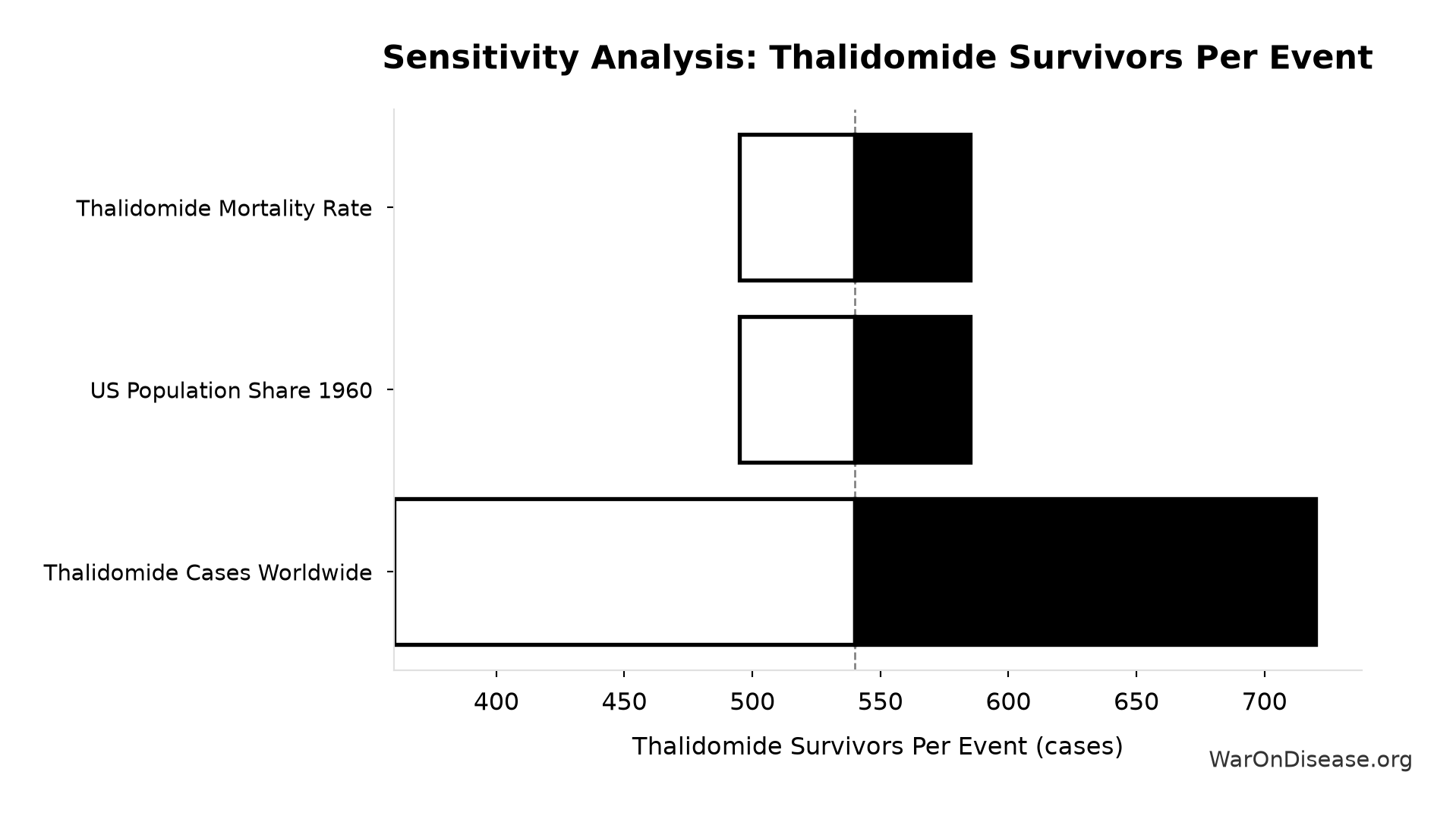
Sensitivity Indices for Thalidomide Survivors Per Event
Regression-based sensitivity showing which inputs explain the most variance in the output.
| Input Parameter | Sensitivity Coefficient | Interpretation |
|---|---|---|
| Thalidomide US Cases Prevented (cases) | 0.9700 | Strong driver |
| Thalidomide Mortality Rate (percentage) | -0.2364 | Weak driver |
Interpretation: Standardized coefficients show the change in output (in SD units) per 1 SD change in input. Values near ±1 indicate strong influence; values exceeding ±1 may occur with correlated inputs.
Monte Carlo Distribution
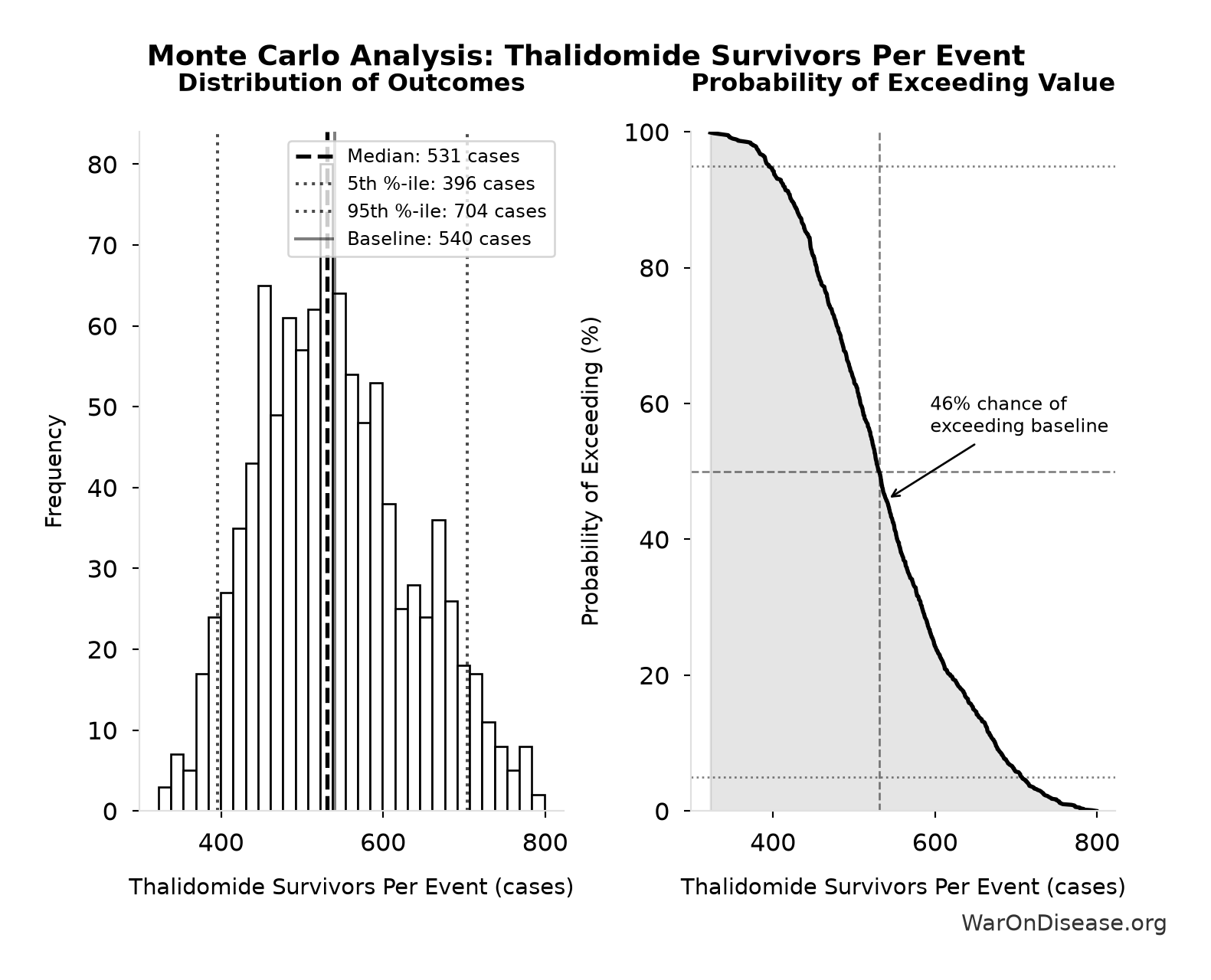
Simulation Results Summary: Thalidomide Survivors Per Event
| Statistic | Value |
|---|---|
| Baseline (deterministic) | 540 |
| Mean (expected value) | 538 |
| Median (50th percentile) | 531 |
| Standard Deviation | 92.5 |
| 90% Range (5th-95th percentile) | [396, 704] |
The histogram shows 1,000 of the 10,000 Monte Carlo draws for Thalidomide Survivors Per Event; the summary statistics use all 10,000. The exceedance curve (right) shows the probability of the outcome exceeding any given value.
Exceedance Probability
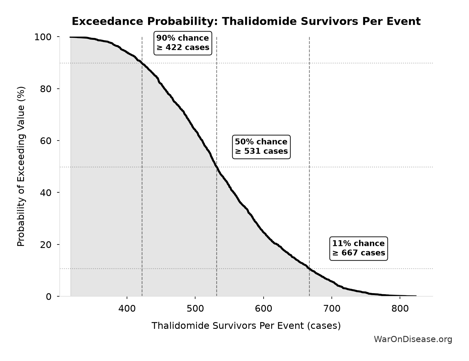
This exceedance probability chart shows the likelihood that Thalidomide Survivors Per Event will exceed any given threshold. The higher the curve at a threshold, the more likely the value exceeds it.
Thalidomide US Cases Prevented: 900 cases
Note📊 Details
Estimated US thalidomide cases prevented by FDA rejection
Inputs:
- Thalidomide Cases Worldwide 📊: 15,000 cases (95% CI: 10,000 cases - 20,000 cases)
- US Population Share 1960 📊: 6% (95% CI: 5.5% - 6.5%)
\[ \begin{gathered} N_{thal,US,prevent} \\ = N_{thal,global} \times Pct_{US,1960} \\ = 15{,}000 \times 6\% \\ = 900 \end{gathered} \]
~ Medium confidence
Sensitivity Analysis
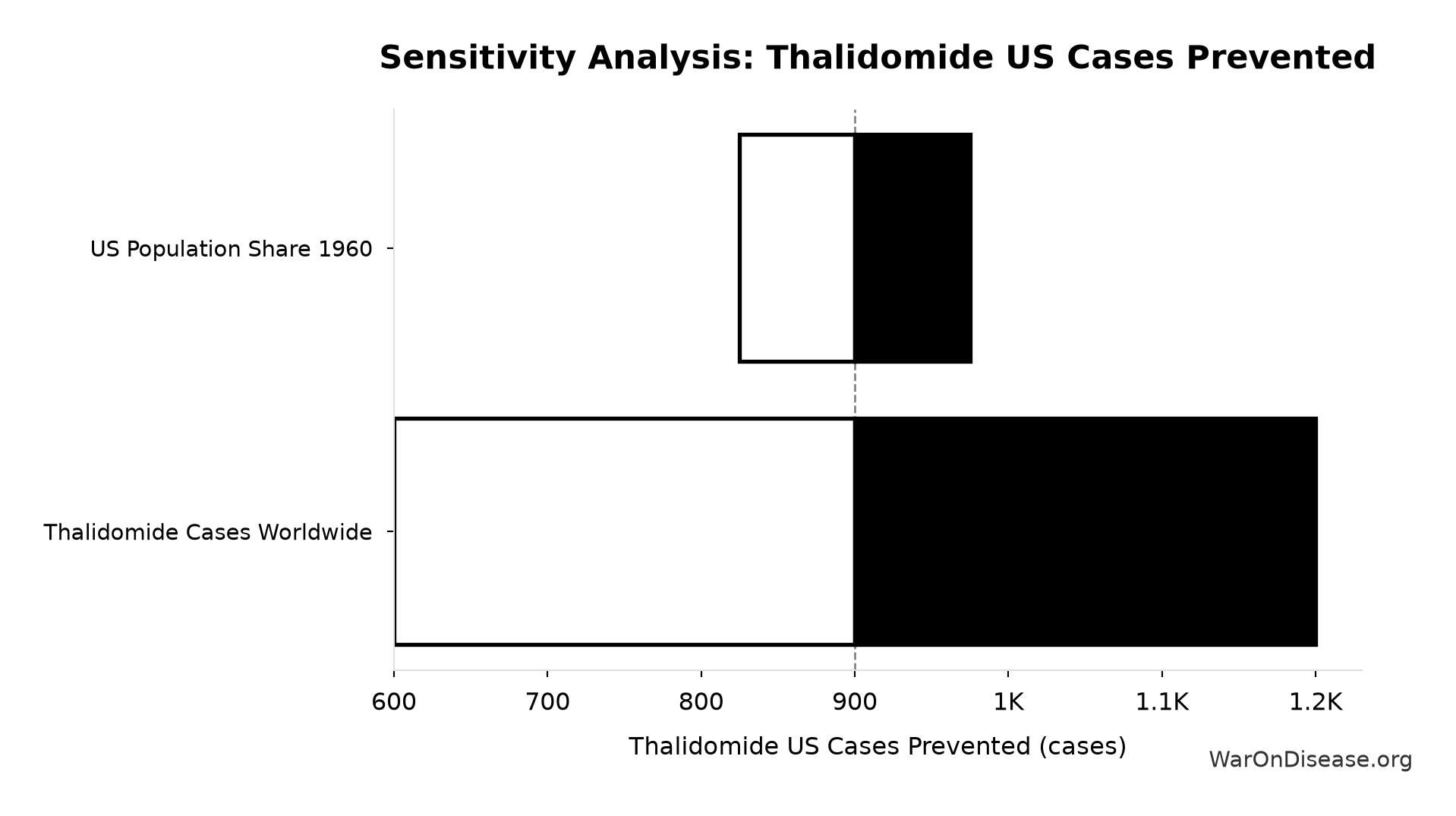
Sensitivity Indices for Thalidomide US Cases Prevented
Regression-based sensitivity showing which inputs explain the most variance in the output.
| Input Parameter | Sensitivity Coefficient | Interpretation |
|---|---|---|
| Thalidomide Cases Worldwide (cases) | 0.9707 | Strong driver |
| US Population Share 1960 (percentage) | 0.2437 | Weak driver |
Interpretation: Standardized coefficients show the change in output (in SD units) per 1 SD change in input. Values near ±1 indicate strong influence; values exceeding ±1 may occur with correlated inputs.
Monte Carlo Distribution
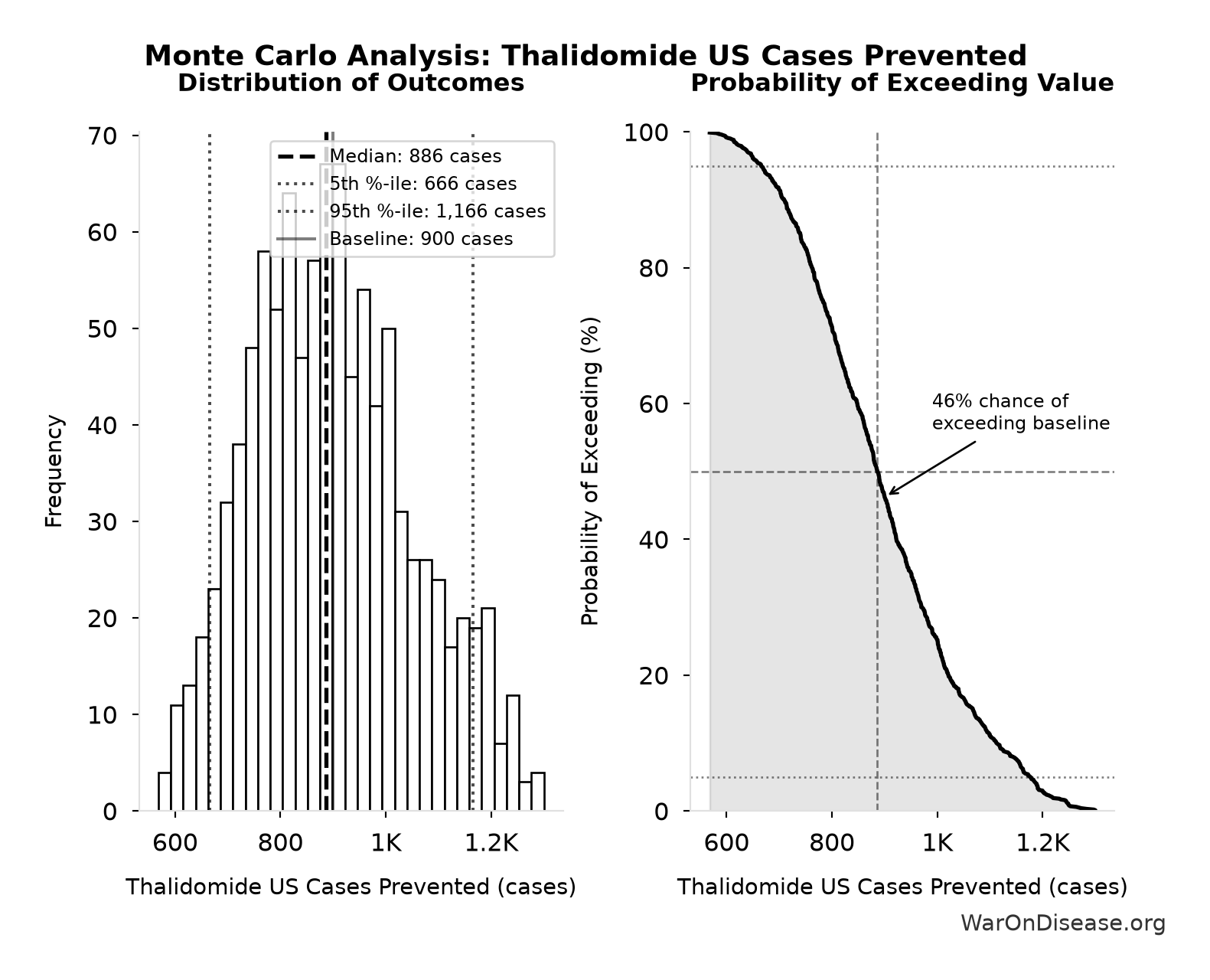
Simulation Results Summary: Thalidomide US Cases Prevented
| Statistic | Value |
|---|---|
| Baseline (deterministic) | 900 |
| Mean (expected value) | 897 |
| Median (50th percentile) | 886 |
| Standard Deviation | 149 |
| 90% Range (5th-95th percentile) | [666, 1,166] |
The histogram shows 1,000 of the 10,000 Monte Carlo draws for Thalidomide US Cases Prevented; the summary statistics use all 10,000. The exceedance curve (right) shows the probability of the outcome exceeding any given value.
Exceedance Probability
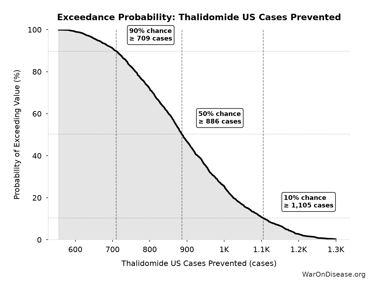
This exceedance probability chart shows the likelihood that Thalidomide US Cases Prevented will exceed any given threshold. The higher the curve at a threshold, the more likely the value exceeds it.
Thalidomide YLD Per Event: 12,960 years
Note📊 Details
Years Lived with Disability per thalidomide event
Inputs:
- Thalidomide Disability Weight 📊: 0.4:1 (95% CI: 0.32:1 - 0.48:1)
- Thalidomide Survivors Per Event 🔢: 540 cases
- Thalidomide Survivor Lifespan 📊: 60 years (95% CI: 50 years - 70 years)
\[ \begin{gathered} YLD_{thal} \\ = DW_{thal} \times N_{thal,survive} \times LE_{thal} \\ = 0.4 \times 540 \times 60 \\ = 13{,}000 \end{gathered} \] where: \[ \begin{gathered} N_{thal,survive} \\ = N_{thal,US,prevent} \times (1 - Rate_{thal,mort}) \\ = 900 \times (1 - 40\%) \\ = 540 \end{gathered} \] where: \[ \begin{gathered} N_{thal,US,prevent} \\ = N_{thal,global} \times Pct_{US,1960} \\ = 15{,}000 \times 6\% \\ = 900 \end{gathered} \] ~ Medium confidence
Sensitivity Analysis
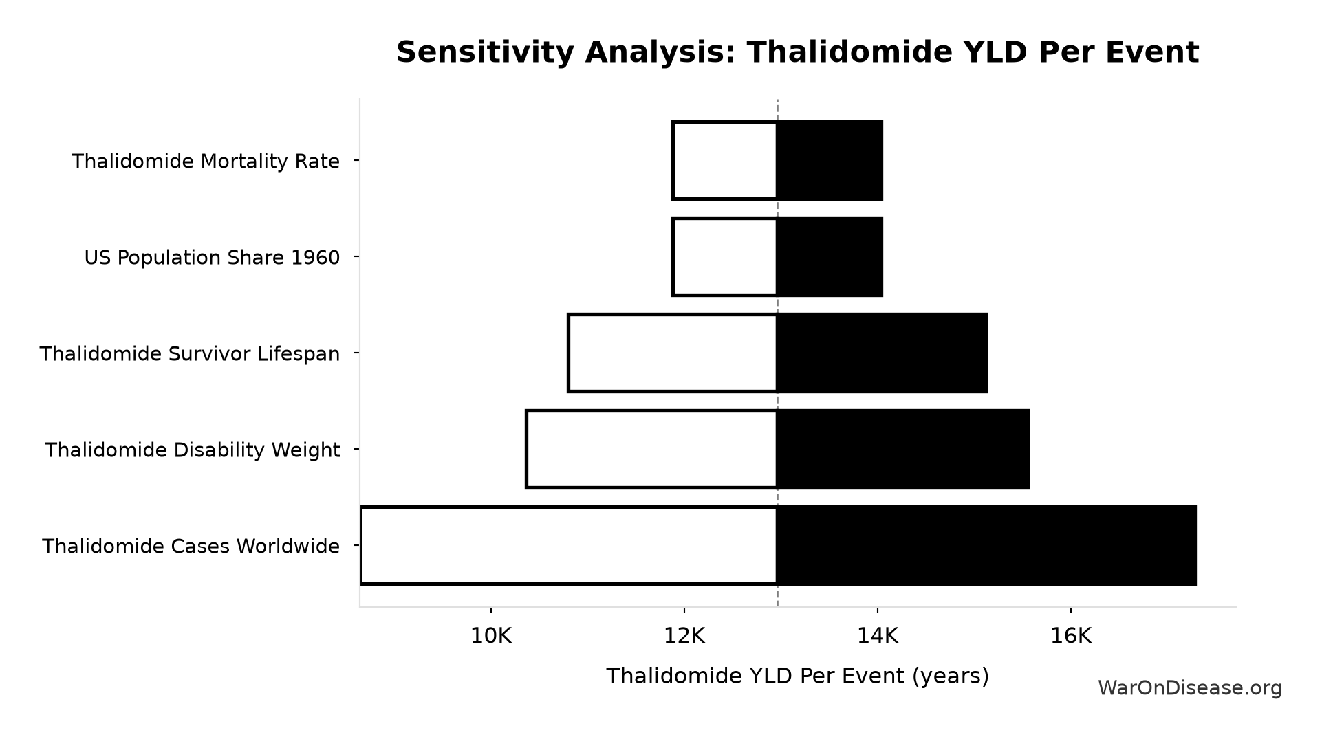
Sensitivity Indices for Thalidomide YLD Per Event
Regression-based sensitivity showing which inputs explain the most variance in the output.
| Input Parameter | Sensitivity Coefficient | Interpretation |
|---|---|---|
| Thalidomide Survivors Per Event (cases) | 0.7990 | Strong driver |
| Thalidomide Disability Weight (ratio) | 0.4526 | Moderate driver |
| Thalidomide Survivor Lifespan (years) | 0.3747 | Moderate driver |
Interpretation: Standardized coefficients show the change in output (in SD units) per 1 SD change in input. Values near ±1 indicate strong influence; values exceeding ±1 may occur with correlated inputs.
Monte Carlo Distribution
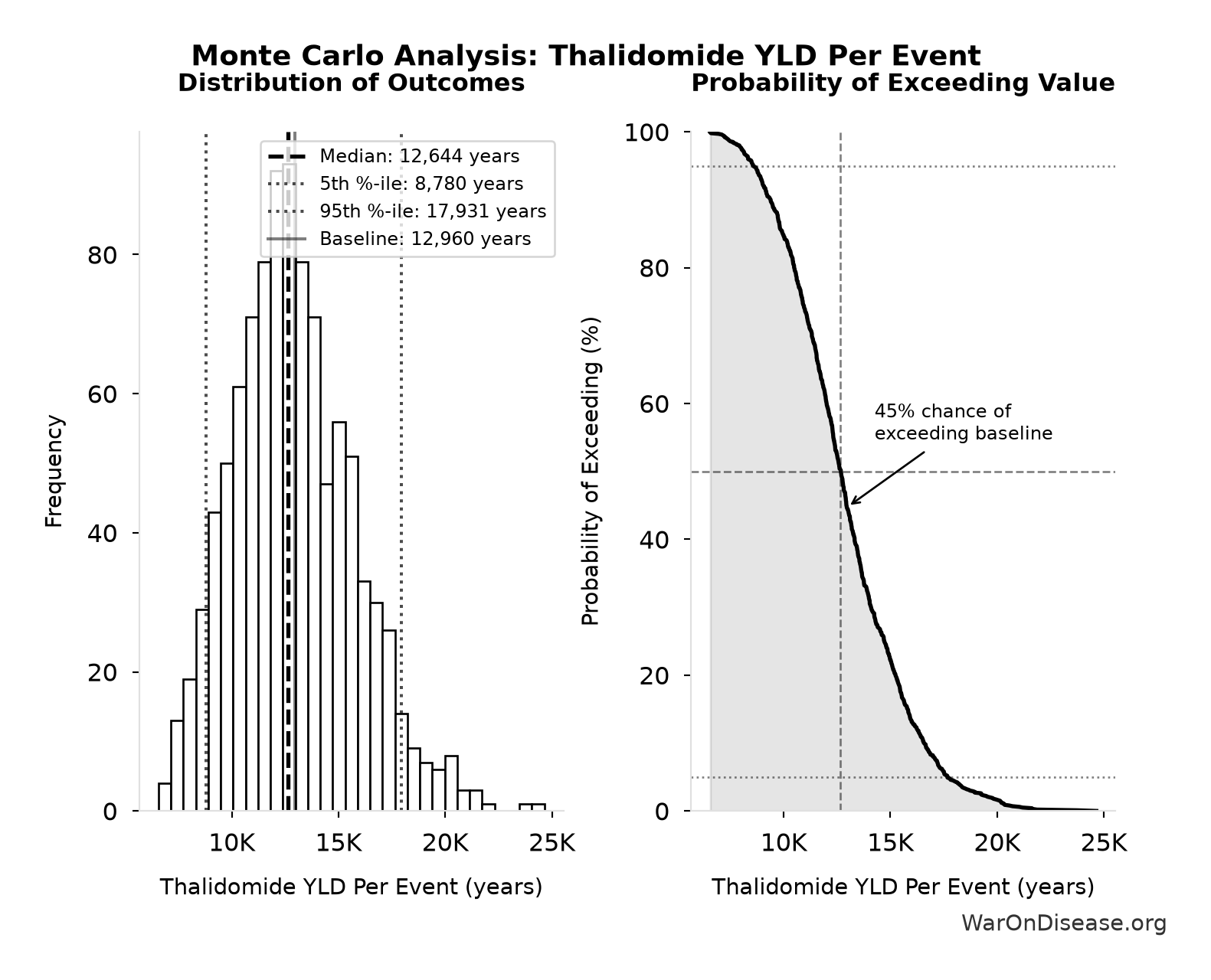
Simulation Results Summary: Thalidomide YLD Per Event
| Statistic | Value |
|---|---|
| Baseline (deterministic) | 12,960 |
| Mean (expected value) | 12,907 |
| Median (50th percentile) | 12,644 |
| Standard Deviation | 2,776 |
| 90% Range (5th-95th percentile) | [8,780, 17,931] |
The histogram shows 1,000 of the 10,000 Monte Carlo draws for Thalidomide YLD Per Event; the summary statistics use all 10,000. The exceedance curve (right) shows the probability of the outcome exceeding any given value.
Exceedance Probability
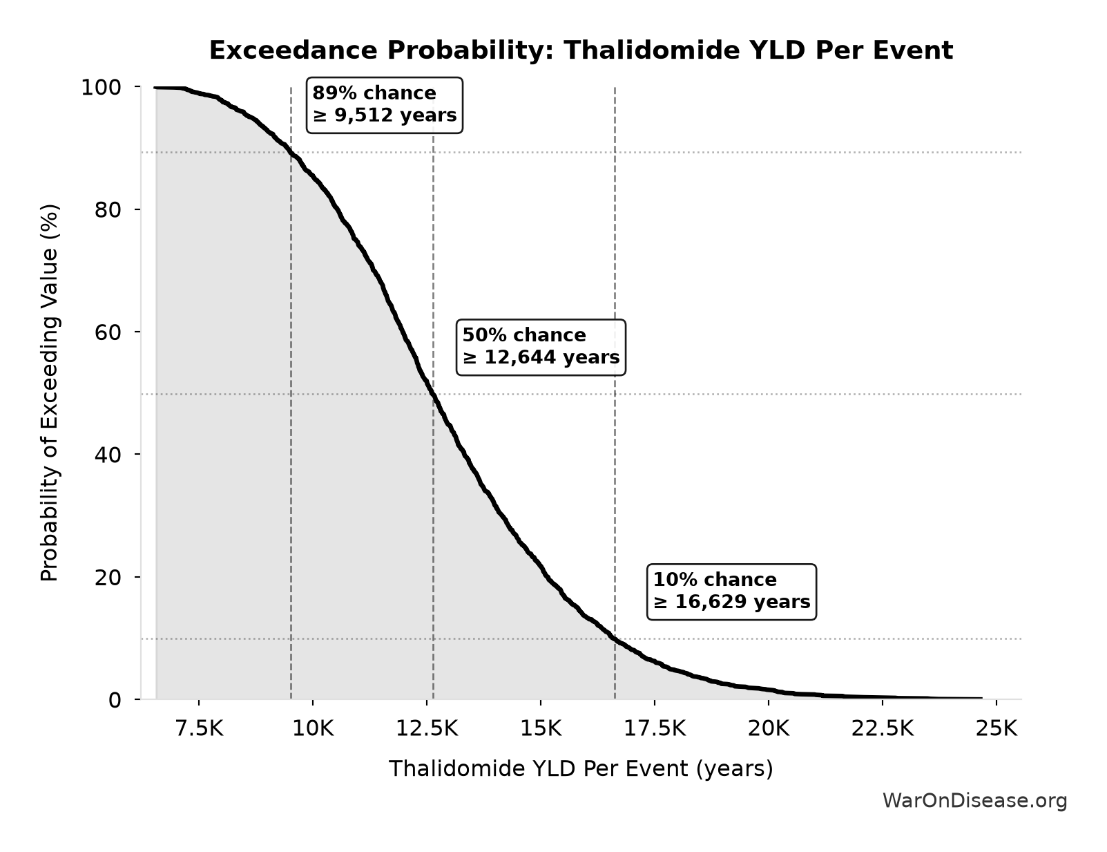
This exceedance probability chart shows the likelihood that Thalidomide YLD Per Event will exceed any given threshold. The higher the curve at a threshold, the more likely the value exceeds it.
Thalidomide YLL Per Event: 28,800 years
Note📊 Details
Years of Life Lost per thalidomide event (infant deaths)
Inputs:
- Thalidomide Deaths Per Event 🔢: 360 deaths
\[ \begin{gathered} YLL_{thal} \\ = Deaths_{thal} \times 80 \\ = 360 \times 80 \\ = 28{,}800 \end{gathered} \] where: \[ \begin{gathered} Deaths_{thal} \\ = Rate_{thal,mort} \times N_{thal,US,prevent} \\ = 40\% \times 900 \\ = 360 \end{gathered} \] where: \[ \begin{gathered} N_{thal,US,prevent} \\ = N_{thal,global} \times Pct_{US,1960} \\ = 15{,}000 \times 6\% \\ = 900 \end{gathered} \] ~ Medium confidence
Sensitivity Analysis
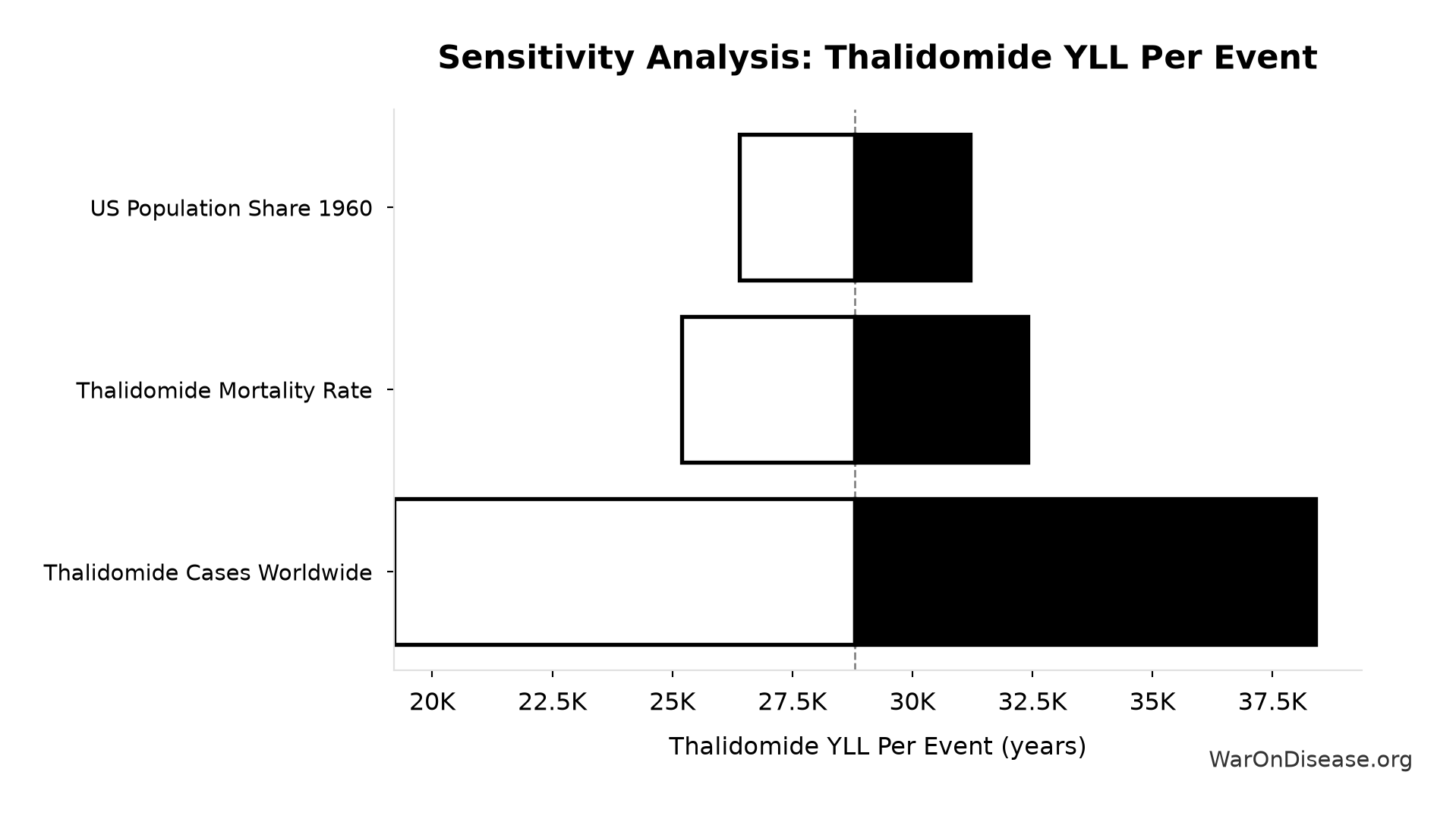
Sensitivity Indices for Thalidomide YLL Per Event
Regression-based sensitivity showing which inputs explain the most variance in the output.
| Input Parameter | Sensitivity Coefficient | Interpretation |
|---|---|---|
| Thalidomide Deaths Per Event (deaths) | 1.0000 | Strong driver |
Interpretation: Standardized coefficients show the change in output (in SD units) per 1 SD change in input. Values near ±1 indicate strong influence; values exceeding ±1 may occur with correlated inputs.
Monte Carlo Distribution
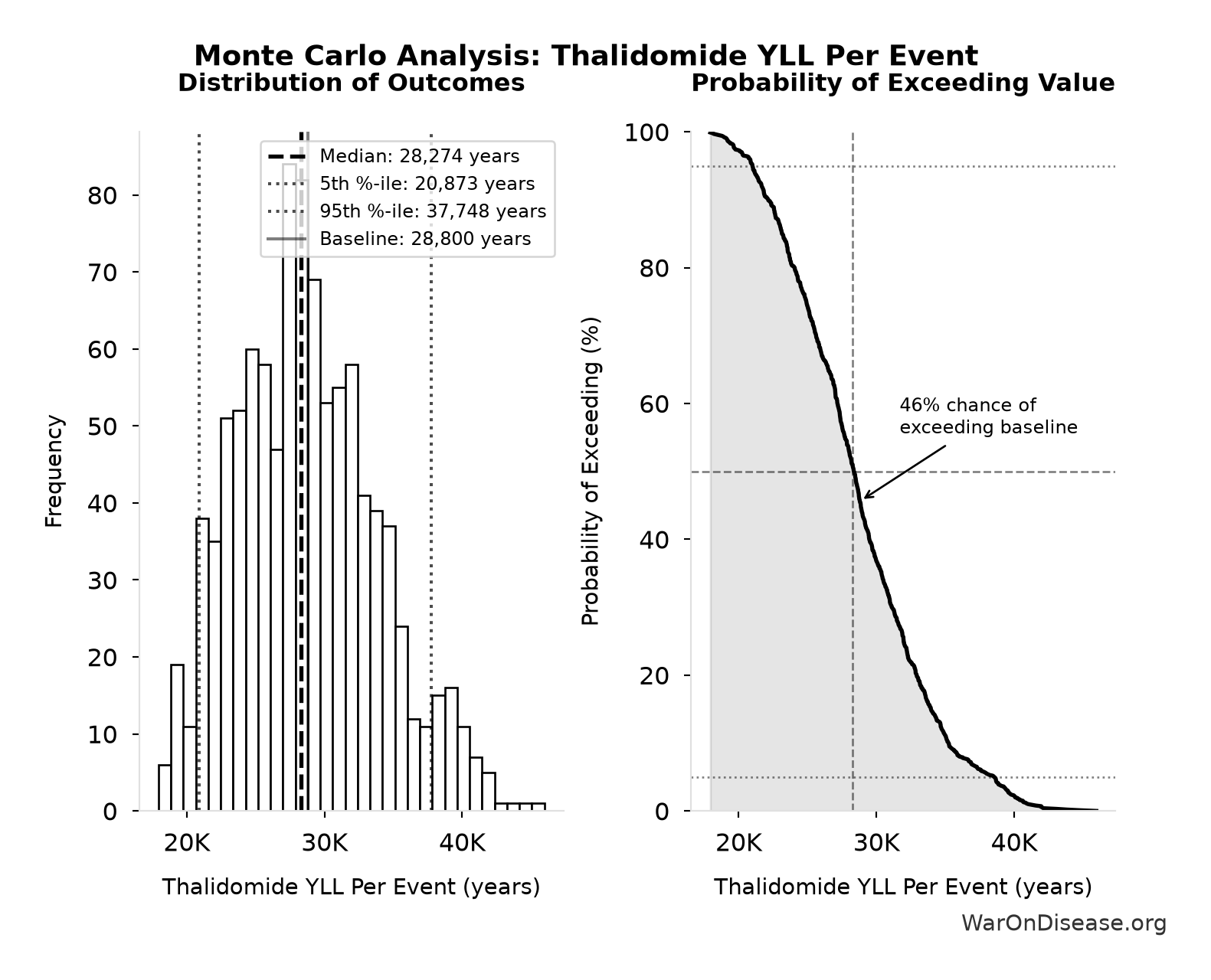
Simulation Results Summary: Thalidomide YLL Per Event
| Statistic | Value |
|---|---|
| Baseline (deterministic) | 28,800 |
| Mean (expected value) | 28,684 |
| Median (50th percentile) | 28,274 |
| Standard Deviation | 5,088 |
| 90% Range (5th-95th percentile) | [20,873, 37,748] |
The histogram shows 1,000 of the 10,000 Monte Carlo draws for Thalidomide YLL Per Event; the summary statistics use all 10,000. The exceedance curve (right) shows the probability of the outcome exceeding any given value.
Exceedance Probability
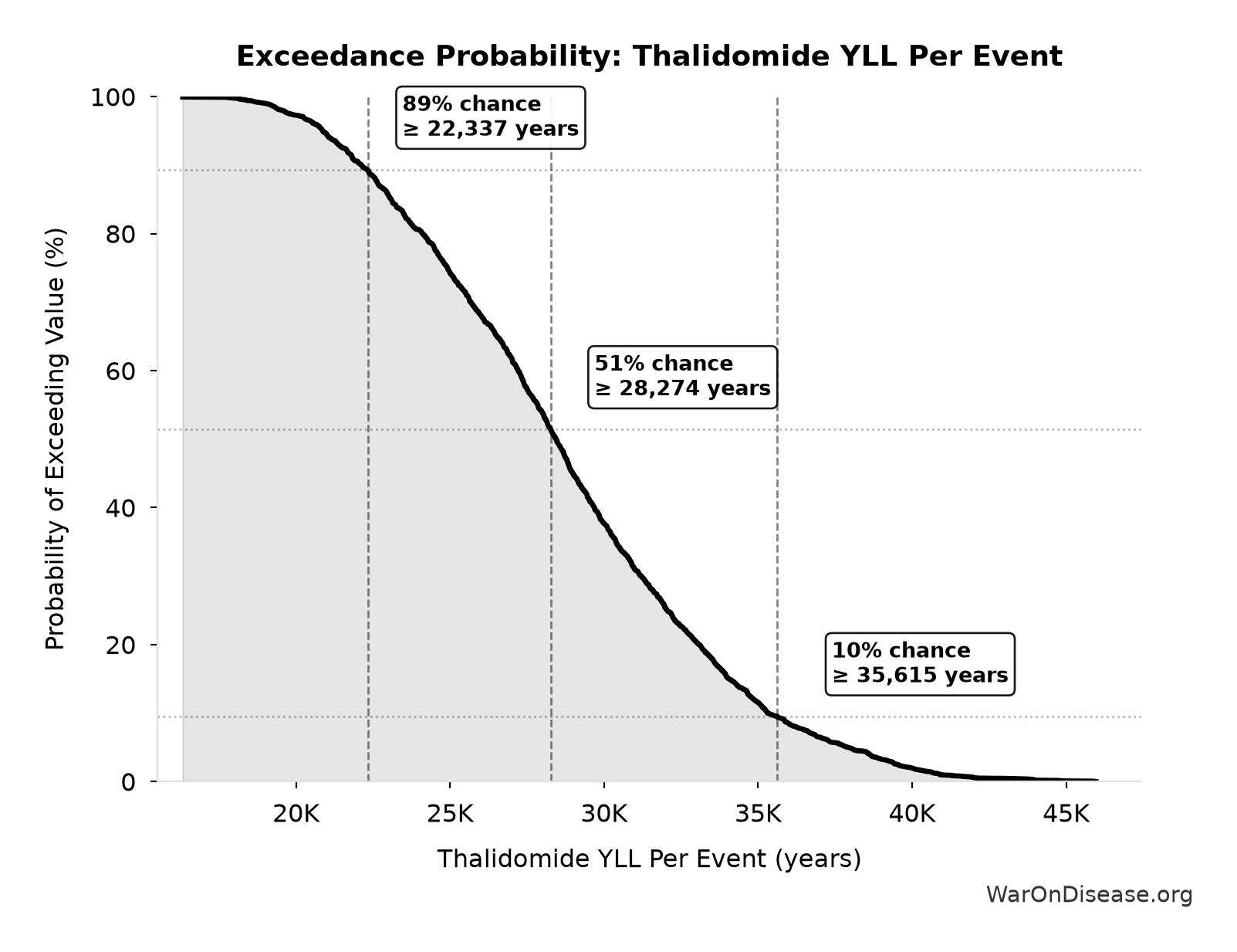
This exceedance probability chart shows the likelihood that Thalidomide YLL Per Event will exceed any given threshold. The higher the curve at a threshold, the more likely the value exceeds it.
Ratio of Type II Error Cost to Type I Error Benefit: 3,389:1
Note📊 Details
Ratio of Type II error cost to Type I error benefit (harm from delay vs. harm prevented)
Inputs:
- Total DALYs Lost from Disease Eradication Delay 🔢: 8.77 billion DALYs
- Maximum DALYs Saved by FDA Preventing Unsafe Drugs (1962-2024) 🔢: 2.59 million DALYs
\[ \begin{gathered} Ratio_{TypeII} \\ = \frac{DALYs_{lag}}{DALY_{TypeI}} \\ = \frac{8.77B}{2.59M} \\ = 3{,}390 \end{gathered} \] where: \[ DALYs_{lag} = YLL_{lag} + YLD_{lag} = 7.9B + 873M = 8.77B \] where: \[ \begin{gathered} YLL_{lag} \\ = \text{DEATHS\_TOTAL} \times (REMAINING_LIFE_EXPECTANCY_AT_60 - (\text{MEAN\_AGE\_OF\_DEATH} - 60)) \end{gathered} \] where: \[ \begin{gathered} Deaths_{lag} \\ = T_{lag} \times Deaths_{disease,daily} \times 338 \\ = 8.2 \times 150{,}000 \times 338 \\ = 416M \end{gathered} \] where: \[ \begin{gathered} YLD_{lag} \\ = Deaths_{lag} \times T_{suffering} \times DW_{chronic} \\ = 416M \times 6 \times 0.35 \\ = 873M \end{gathered} \] where: \[ \begin{gathered} DALY_{TypeI} \\ = DALY_{thal} \times 62 \\ = 41{,}800 \times 62 \\ = 2.59M \end{gathered} \] where: \[ \begin{gathered} DALY_{thal} \\ = YLD_{thal} + YLL_{thal} \\ = 13{,}000 + 28{,}800 \\ = 41{,}800 \end{gathered} \] where: \[ \begin{gathered} YLD_{thal} \\ = DW_{thal} \times N_{thal,survive} \times LE_{thal} \\ = 0.4 \times 540 \times 60 \\ = 13{,}000 \end{gathered} \] where: \[ \begin{gathered} N_{thal,survive} \\ = N_{thal,US,prevent} \times (1 - Rate_{thal,mort}) \\ = 900 \times (1 - 40\%) \\ = 540 \end{gathered} \] where: \[ \begin{gathered} N_{thal,US,prevent} \\ = N_{thal,global} \times Pct_{US,1960} \\ = 15{,}000 \times 6\% \\ = 900 \end{gathered} \] where: \[ \begin{gathered} YLL_{thal} \\ = Deaths_{thal} \times 80 \\ = 360 \times 80 \\ = 28{,}800 \end{gathered} \] where: \[ \begin{gathered} Deaths_{thal} \\ = Rate_{thal,mort} \times N_{thal,US,prevent} \\ = 40\% \times 900 \\ = 360 \end{gathered} \] ~ Medium confidence
Sensitivity Analysis
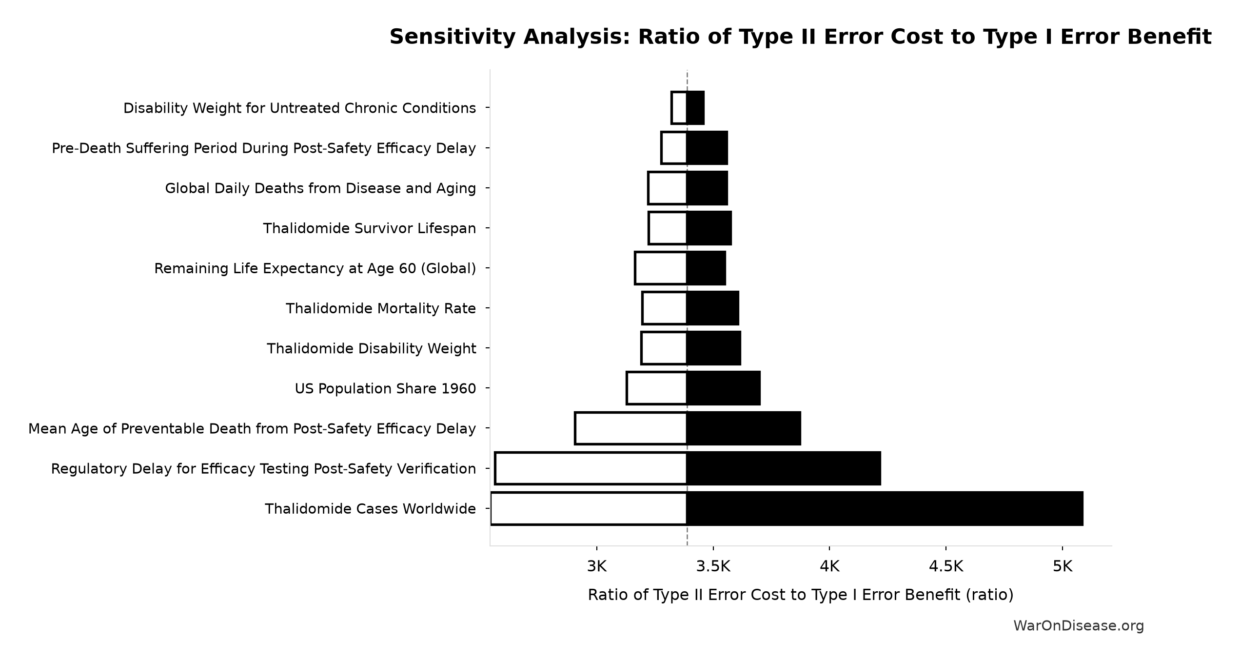
Sensitivity Indices for Ratio of Type II Error Cost to Type I Error Benefit
Regression-based sensitivity showing which inputs explain the most variance in the output.
| Input Parameter | Sensitivity Coefficient | Interpretation |
|---|---|---|
| Total DALYs Lost from Disease Eradication Delay (DALYs) | 0.8413 | Strong driver |
| Maximum DALYs Saved by FDA Preventing Unsafe Drugs (1962-2024) (DALYs) | -0.4986 | Moderate driver |
Interpretation: Standardized coefficients show the change in output (in SD units) per 1 SD change in input. Values near ±1 indicate strong influence; values exceeding ±1 may occur with correlated inputs.
Monte Carlo Distribution
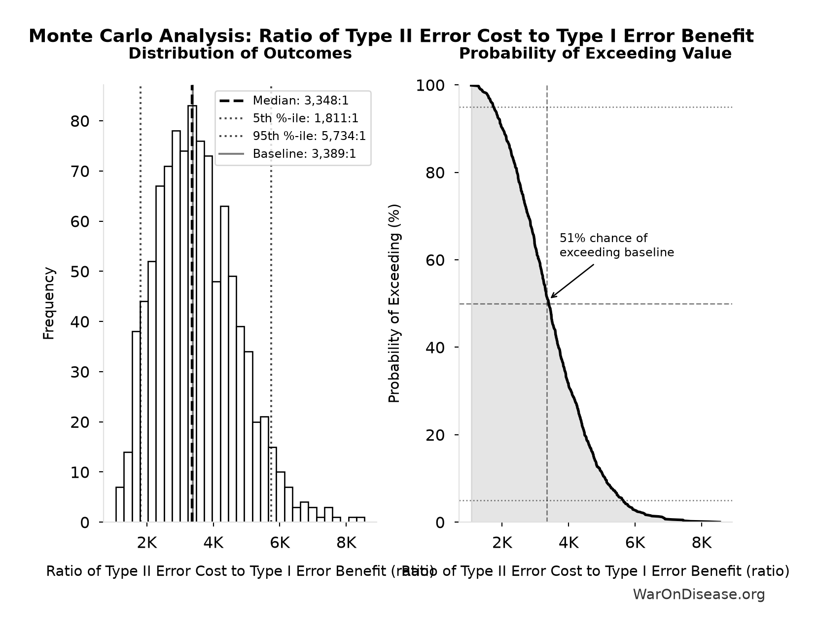
Simulation Results Summary: Ratio of Type II Error Cost to Type I Error Benefit
| Statistic | Value |
|---|---|
| Baseline (deterministic) | 3,389:1 |
| Mean (expected value) | 3,510:1 |
| Median (50th percentile) | 3,348:1 |
| Standard Deviation | 1,215:1 |
| 90% Range (5th-95th percentile) | [1,811:1, 5,734:1] |
The histogram shows 1,000 of the 10,000 Monte Carlo draws for Ratio of Type II Error Cost to Type I Error Benefit; the summary statistics use all 10,000. The exceedance curve (right) shows the probability of the outcome exceeding any given value.
Exceedance Probability
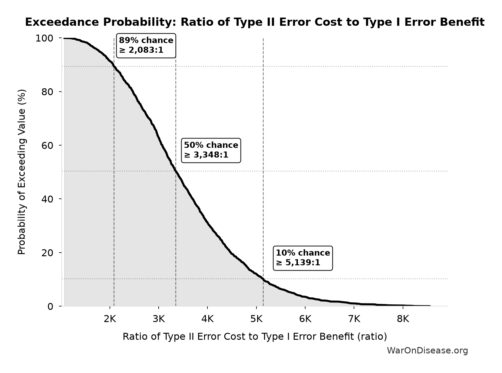
This exceedance probability chart shows the likelihood that Ratio of Type II Error Cost to Type I Error Benefit will exceed any given threshold. The higher the curve at a threshold, the more likely the value exceeds it.
Maximum DALYs Saved by FDA Preventing Unsafe Drugs (1962-2024): 2.59 million DALYs
Note📊 Details
Maximum DALYs saved by FDA preventing unsafe drugs over 62-year period 1962-2024 (extreme overestimate: one Thalidomide-scale event per year)
Inputs:
- Thalidomide DALYs Per Event 🔢: 41,760 DALYs
\[ \begin{gathered} DALY_{TypeI} \\ = DALY_{thal} \times 62 \\ = 41{,}800 \times 62 \\ = 2.59M \end{gathered} \] where: \[ \begin{gathered} DALY_{thal} \\ = YLD_{thal} + YLL_{thal} \\ = 13{,}000 + 28{,}800 \\ = 41{,}800 \end{gathered} \] where: \[ \begin{gathered} YLD_{thal} \\ = DW_{thal} \times N_{thal,survive} \times LE_{thal} \\ = 0.4 \times 540 \times 60 \\ = 13{,}000 \end{gathered} \] where: \[ \begin{gathered} N_{thal,survive} \\ = N_{thal,US,prevent} \times (1 - Rate_{thal,mort}) \\ = 900 \times (1 - 40\%) \\ = 540 \end{gathered} \] where: \[ \begin{gathered} N_{thal,US,prevent} \\ = N_{thal,global} \times Pct_{US,1960} \\ = 15{,}000 \times 6\% \\ = 900 \end{gathered} \] where: \[ \begin{gathered} YLL_{thal} \\ = Deaths_{thal} \times 80 \\ = 360 \times 80 \\ = 28{,}800 \end{gathered} \] where: \[ \begin{gathered} Deaths_{thal} \\ = Rate_{thal,mort} \times N_{thal,US,prevent} \\ = 40\% \times 900 \\ = 360 \end{gathered} \] ? Low confidence
Sensitivity Analysis
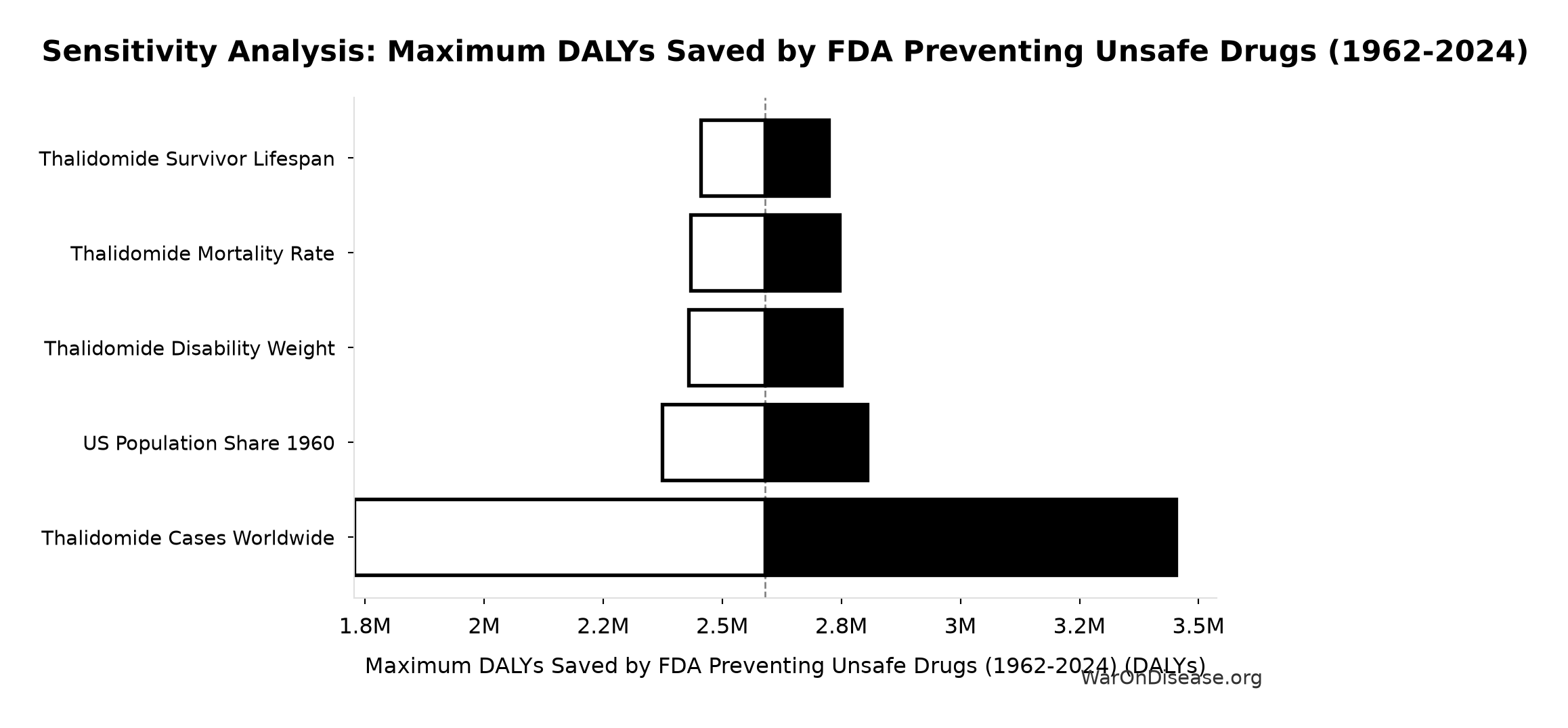
Sensitivity Indices for Maximum DALYs Saved by FDA Preventing Unsafe Drugs (1962-2024)
Regression-based sensitivity showing which inputs explain the most variance in the output.
| Input Parameter | Sensitivity Coefficient | Interpretation |
|---|---|---|
| Thalidomide DALYs Per Event (DALYs) | 1.0000 | Strong driver |
Interpretation: Standardized coefficients show the change in output (in SD units) per 1 SD change in input. Values near ±1 indicate strong influence; values exceeding ±1 may occur with correlated inputs.
Monte Carlo Distribution
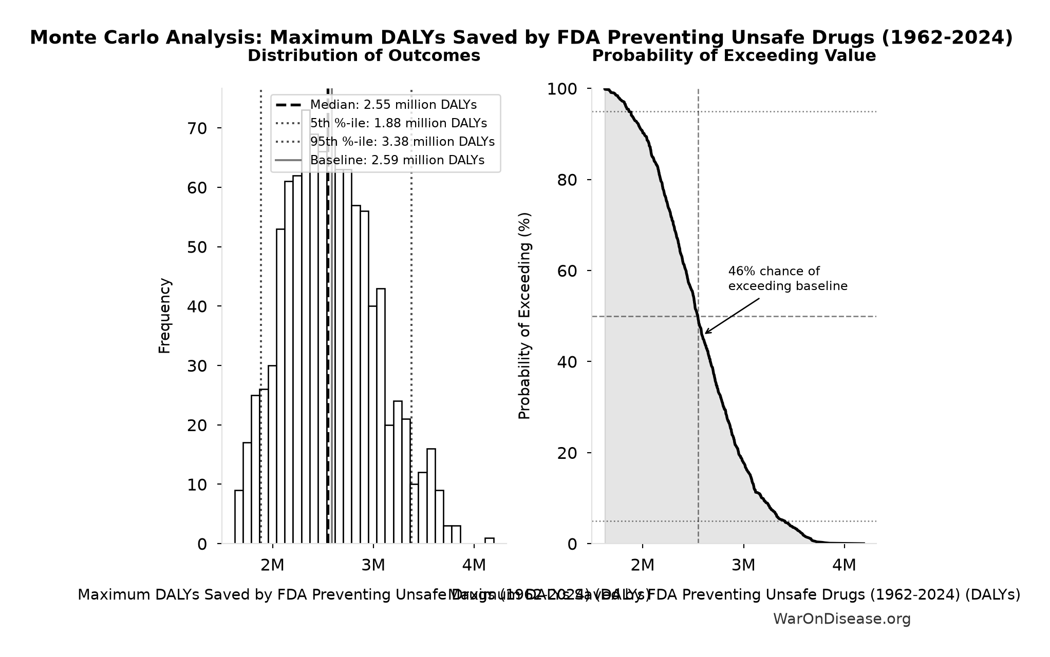
Simulation Results Summary: Maximum DALYs Saved by FDA Preventing Unsafe Drugs (1962-2024)
| Statistic | Value |
|---|---|
| Baseline (deterministic) | 2.59 million |
| Mean (expected value) | 2.58 million |
| Median (50th percentile) | 2.55 million |
| Standard Deviation | 448 thousand |
| 90% Range (5th-95th percentile) | [1.88 million, 3.38 million] |
The histogram shows 1,000 of the 10,000 Monte Carlo draws for Maximum DALYs Saved by FDA Preventing Unsafe Drugs (1962-2024); the summary statistics use all 10,000. The exceedance curve (right) shows the probability of the outcome exceeding any given value.
Exceedance Probability
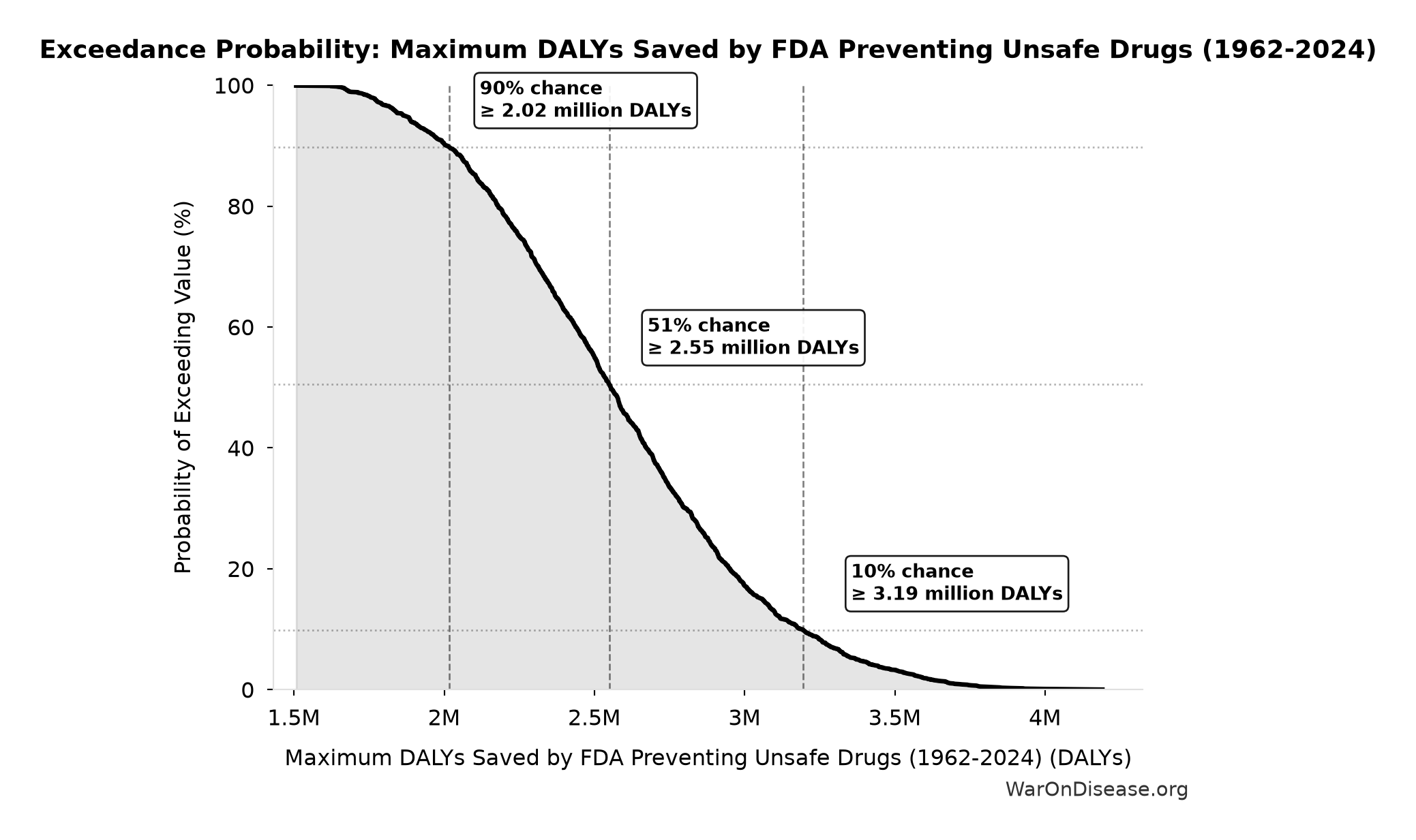
This exceedance probability chart shows the likelihood that Maximum DALYs Saved by FDA Preventing Unsafe Drugs (1962-2024) will exceed any given threshold. The higher the curve at a threshold, the more likely the value exceeds it.
Unexplored Therapeutic Frontier: 99.7%
Note📊 Details
Fraction of possible drug-disease space that remains unexplored (>99%)
Inputs:
- Tested Drug-Disease Relationships: 32,500 relationships (95% CI: 15,000 relationships - 50,000 relationships)
- Possible Drug-Disease Combinations 🔢: 9.5 million combinations
\[ \begin{gathered} Ratio_{unexplored} \\ = 1 - \frac{N_{tested}}{N_{combos}} \\ = 1 - \frac{32{,}500}{9.5M} \\ = 99.7\% \end{gathered} \] where: \[ \begin{gathered} N_{combos} \\ = N_{safe} \times N_{diseases,trial} \\ = 9{,}500 \times 1{,}000 \\ = 9.5M \end{gathered} \] ✓ High confidence
Sensitivity Analysis
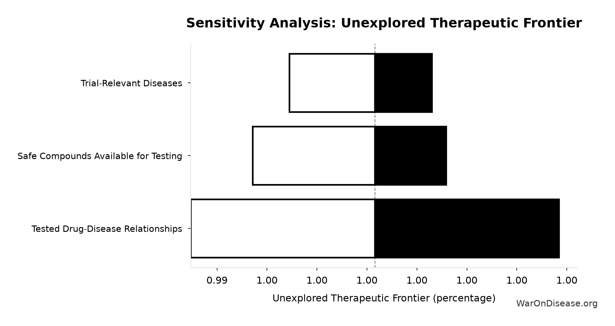
Sensitivity Indices for Unexplored Therapeutic Frontier
Regression-based sensitivity showing which inputs explain the most variance in the output.
| Input Parameter | Sensitivity Coefficient | Interpretation |
|---|---|---|
| Tested Drug-Disease Relationships (relationships) | -0.7794 | Strong driver |
| Possible Drug-Disease Combinations (combinations) | 0.5916 | Strong driver |
Interpretation: Standardized coefficients show the change in output (in SD units) per 1 SD change in input. Values near ±1 indicate strong influence; values exceeding ±1 may occur with correlated inputs.
Monte Carlo Distribution

Simulation Results Summary: Unexplored Therapeutic Frontier
| Statistic | Value |
|---|---|
| Baseline (deterministic) | 99.7% |
| Mean (expected value) | 99.6% |
| Median (50th percentile) | 99.7% |
| Standard Deviation | 0.116% |
| 90% Range (5th-95th percentile) | [99.4%, 99.8%] |
The histogram shows 1,000 of the 10,000 Monte Carlo draws for Unexplored Therapeutic Frontier; the summary statistics use all 10,000. The exceedance curve (right) shows the probability of the outcome exceeding any given value.
Exceedance Probability
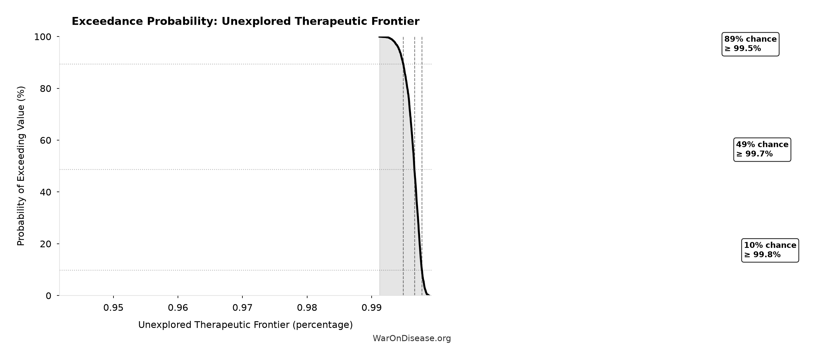
This exceedance probability chart shows the likelihood that Unexplored Therapeutic Frontier will exceed any given threshold. The higher the curve at a threshold, the more likely the value exceeds it.
External Data Sources
Parameters sourced from peer-reviewed publications, institutional databases, and authoritative reports.
ADAPTABLE Trial Cost per Patient: $929
Note📊 Details
Cost per patient in ADAPTABLE trial ($14M PCORI grant / 15,076 patients). Note: This is the direct grant cost; true cost including in-kind may be 10-40% higher.
Source:1
Uncertainty Range
Technical: 95% CI: [$929, $1,400] • Distribution: Lognormal
What this means: There’s significant uncertainty here. The true value likely falls between $929 and $1,400 (±25%). This represents a wide range that our Monte Carlo simulations account for when calculating overall uncertainty in the results.
The lognormal distribution means values can’t go negative and have a longer tail toward higher values (common for costs and populations).
Input Distribution
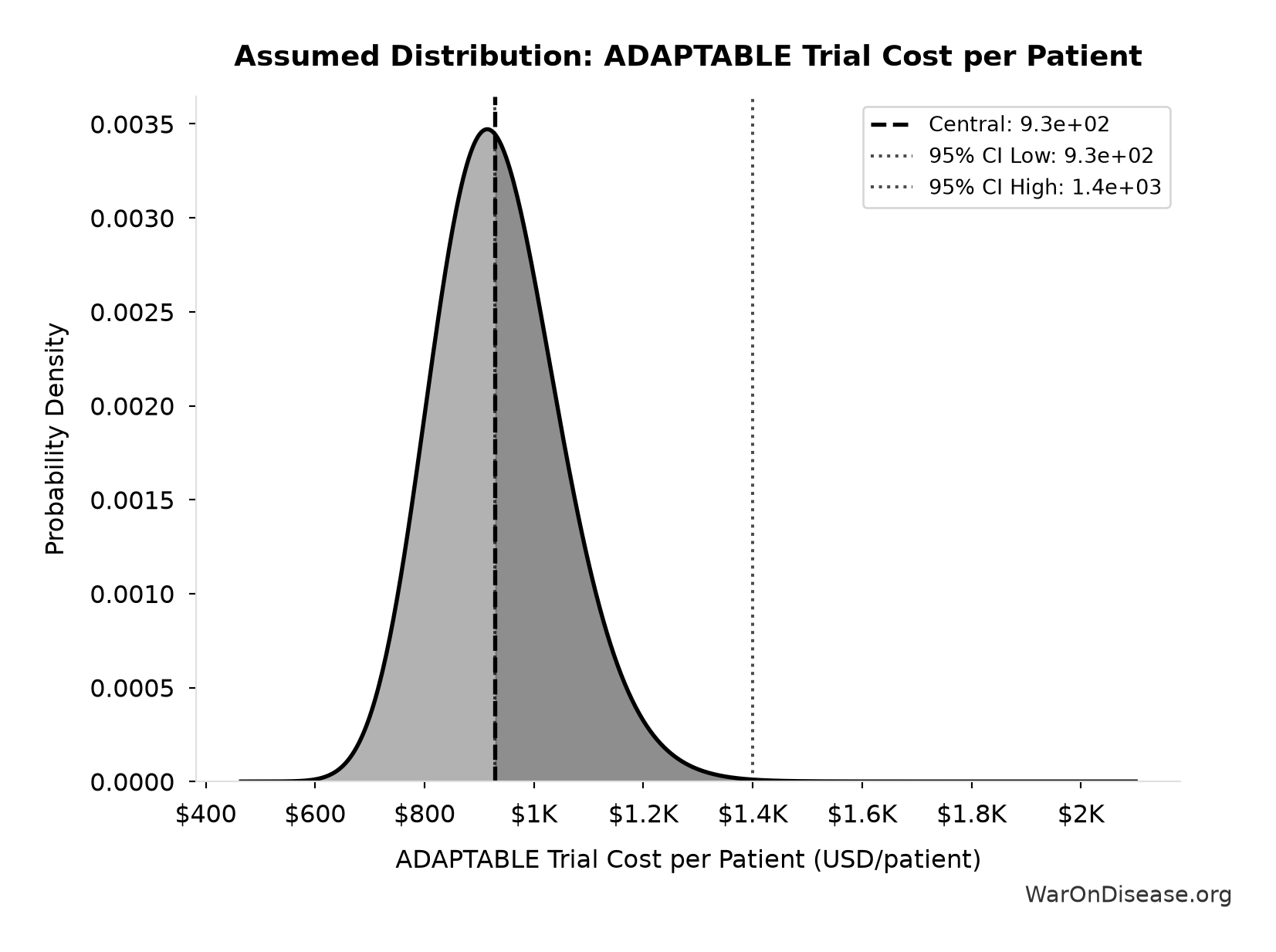
This chart shows the assumed probability distribution for this parameter. The shaded region represents the 95% confidence interval where we expect the true value to fall.
~ Medium confidence
ADAPTABLE Trial Total Cost: $14 million
Note📊 Details
PCORI grant for ADAPTABLE trial (2016-2019). Note: Direct funding only; total costs including site overhead and in-kind contributions from health systems may be higher.
Source:1
Uncertainty Range
Technical: 95% CI: [$14 million, $20 million] • Distribution: Lognormal
What this means: This estimate has moderate uncertainty. The true value likely falls between $14 million and $20 million (±21%). This represents a reasonable range that our Monte Carlo simulations account for when calculating overall uncertainty in the results.
The lognormal distribution means values can’t go negative and have a longer tail toward higher values (common for costs and populations).
Input Distribution
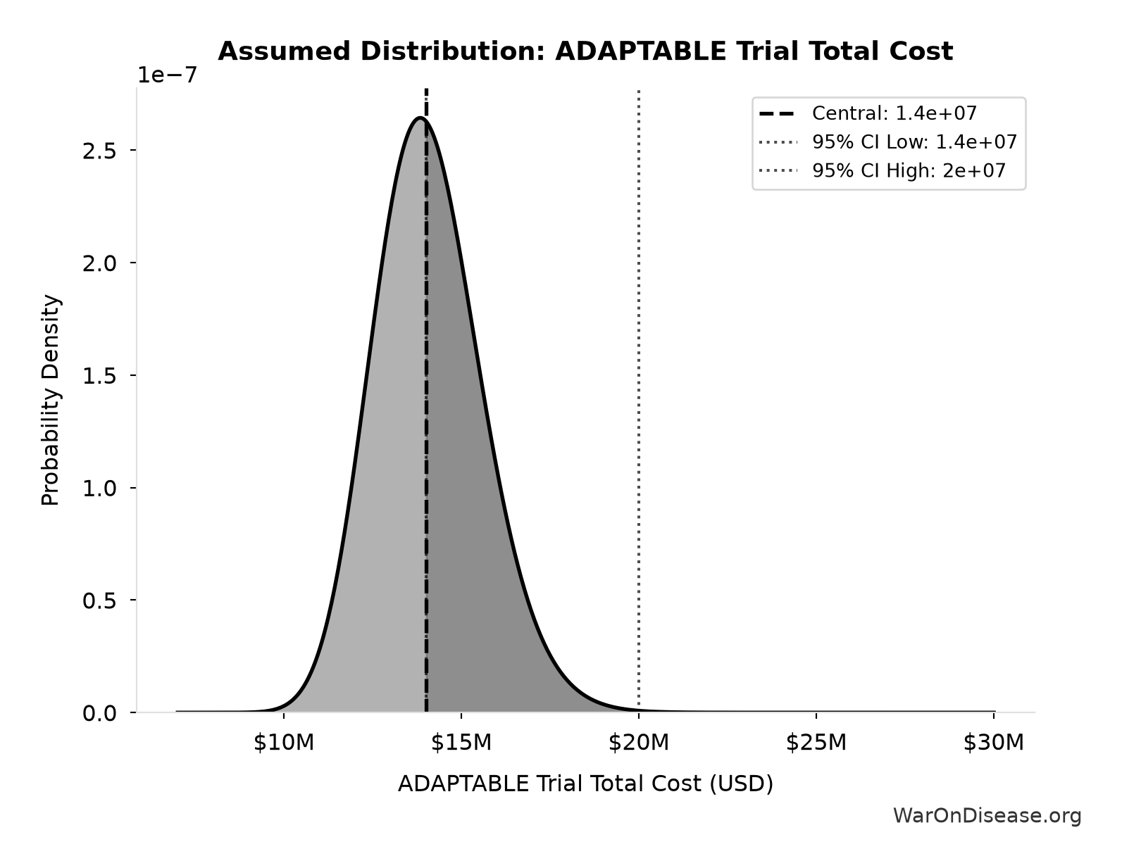
This chart shows the assumed probability distribution for this parameter. The shaded region represents the 95% confidence interval where we expect the true value to fall.
~ Medium confidence
Antidepressant Trial Exclusion Rate: 86.1%
Note📊 Details
Mean exclusion rate in antidepressant trials (86.1% of real-world patients excluded)
Source:2
✓ High confidence
Bed Nets Cost per DALY: $89
Note📊 Details
GiveWell cost per DALY for insecticide-treated bed nets (midpoint estimate, range $78-100). DALYs (Disability-Adjusted Life Years) measure disease burden by combining years of life lost and years lived with disability. Bed nets prevent malaria deaths and are considered a gold standard benchmark for cost-effective global health interventions - if an intervention costs less per DALY than bed nets, it’s exceptionally cost-effective. GiveWell synthesizes peer-reviewed academic research with transparent, rigorous methodology and extensive external expert review.
Source:3
Uncertainty Range
Technical: 95% CI: [$78, $100] • Distribution: Normal
What this means: This estimate has moderate uncertainty. The true value likely falls between $78 and $100 (±12%). This represents a reasonable range that our Monte Carlo simulations account for when calculating overall uncertainty in the results.
The normal distribution means values cluster around the center with equal chances of being higher or lower.
Input Distribution
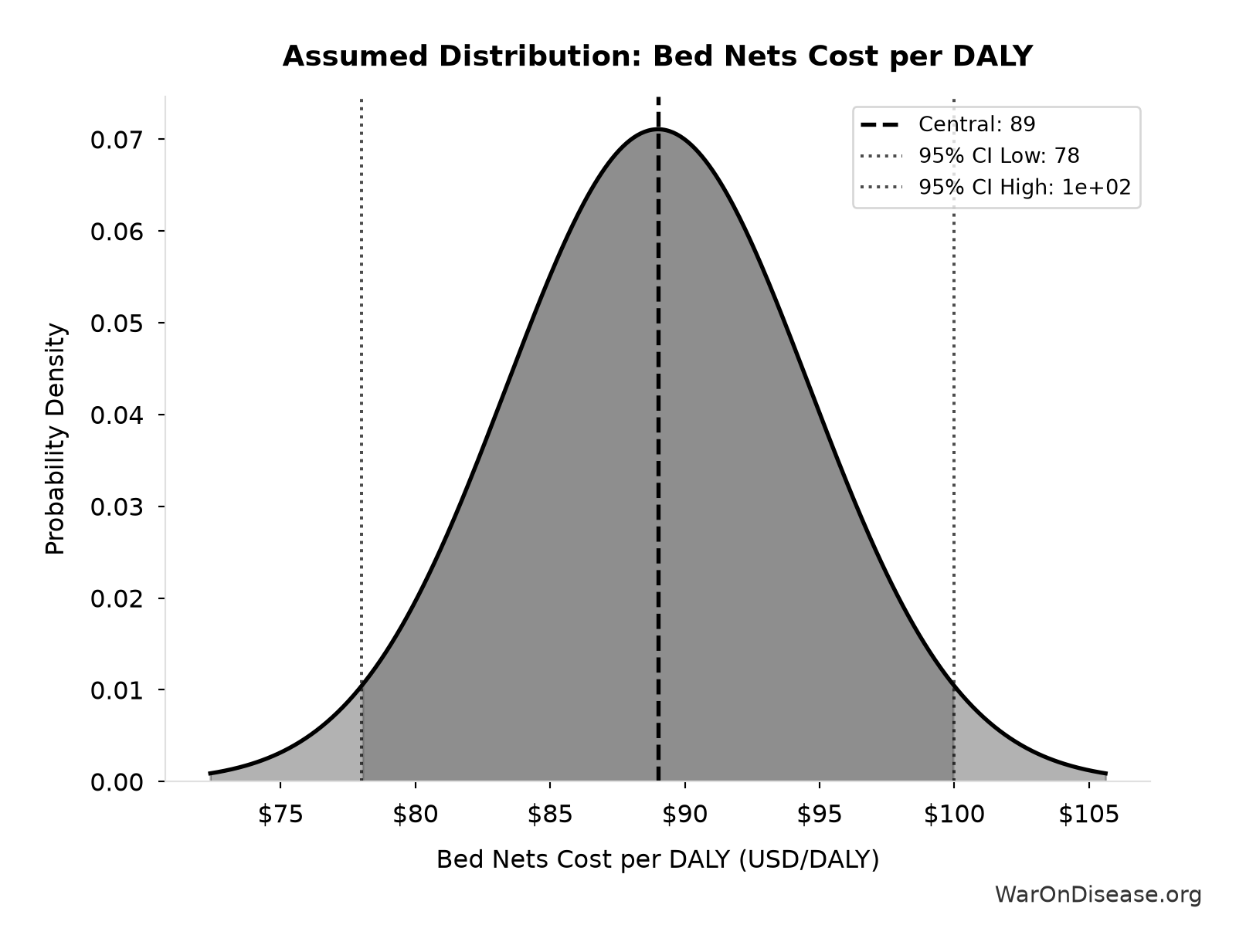
This chart shows the assumed probability distribution for this parameter. The shaded region represents the 95% confidence interval where we expect the true value to fall.
✓ High confidence • 📊 Peer-reviewed
Disability Weight for Untreated Chronic Conditions: 0.35 weight
Note📊 Details
Disability weight for untreated chronic conditions (WHO Global Burden of Disease)
Source:4
Uncertainty Range
Technical: Distribution: Normal (SE: 0.07 weight)
Input Distribution
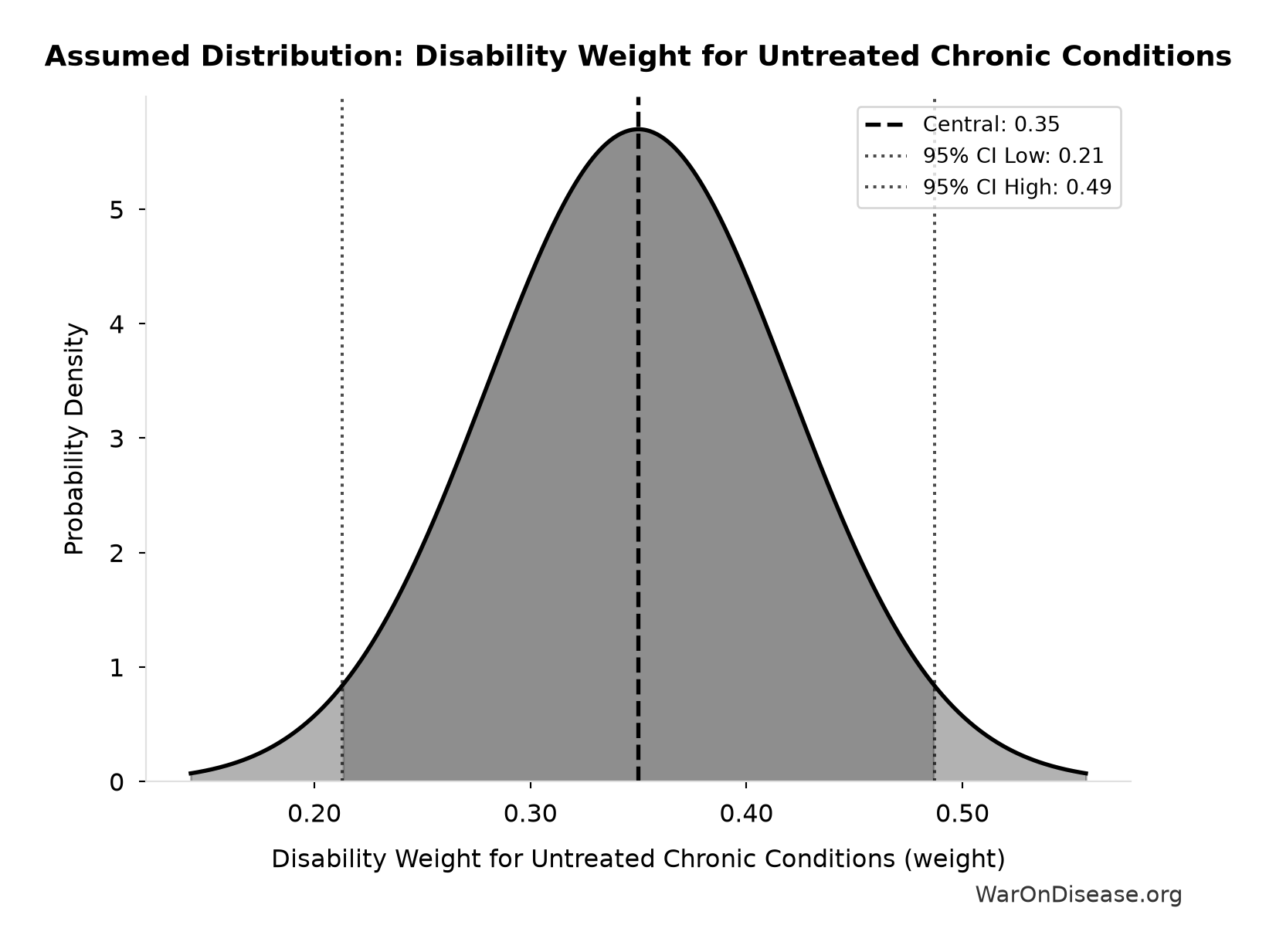
This chart shows the assumed probability distribution for this parameter. The shaded region represents the 95% confidence interval where we expect the true value to fall.
~ Medium confidence • 📊 Peer-reviewed
CPI Multiplier: 1980 to 2024: 3.8:1
Note📊 Details
CPI inflation multiplier from 1980 to 2024 (280.48% cumulative inflation)
Source:5
Uncertainty Range
Technical: 95% CI: [3.75:1, 3.85:1] • Distribution: Normal
What this means: We’re quite confident in this estimate. The true value likely falls between 3.75:1 and 3.85:1 (±1%). This represents a narrow range that our Monte Carlo simulations account for when calculating overall uncertainty in the results.
The normal distribution means values cluster around the center with equal chances of being higher or lower.
Input Distribution
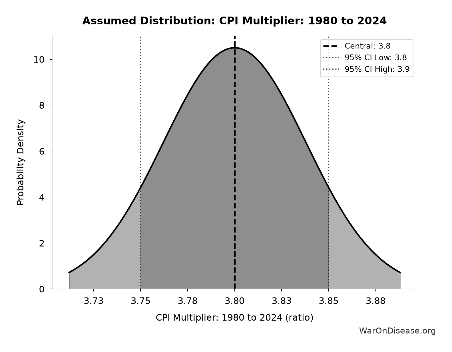
This chart shows the assumed probability distribution for this parameter. The shaded region represents the 95% confidence interval where we expect the true value to fall.
✓ High confidence
Current Clinical Trial Participation Rate: 0.06%
Note📊 Details
Global Population with Chronic Diseases: 2.4 billion people
Note📊 Details
Global population with chronic diseases
Source:7
Uncertainty Range
Technical: 95% CI: [2 billion people, 2.8 billion people] • Distribution: Lognormal
What this means: This estimate has moderate uncertainty. The true value likely falls between 2 billion people and 2.8 billion people (±17%). This represents a reasonable range that our Monte Carlo simulations account for when calculating overall uncertainty in the results.
The lognormal distribution means values can’t go negative and have a longer tail toward higher values (common for costs and populations).
Input Distribution
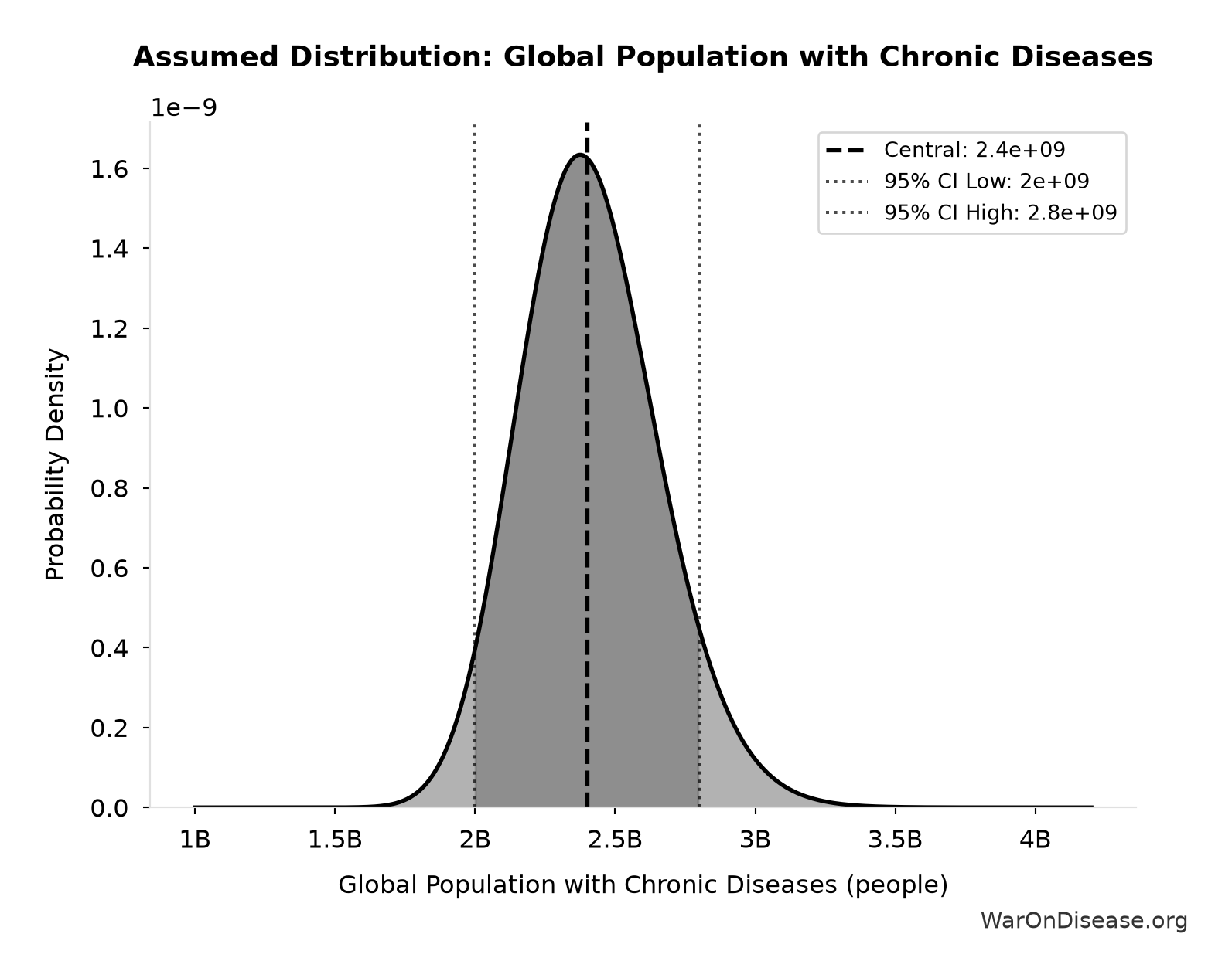
This chart shows the assumed probability distribution for this parameter. The shaded region represents the 95% confidence interval where we expect the true value to fall.
✓ High confidence
Average Annual New Drug Approvals Globally: 50 drugs/year
Note📊 Details
Average annual new drug approvals globally
Source:8
Uncertainty Range
Technical: 95% CI: [45 drugs/year, 60 drugs/year] • Distribution: Lognormal
What this means: This estimate has moderate uncertainty. The true value likely falls between 45 drugs/year and 60 drugs/year (±15%). This represents a reasonable range that our Monte Carlo simulations account for when calculating overall uncertainty in the results.
The lognormal distribution means values can’t go negative and have a longer tail toward higher values (common for costs and populations).
Input Distribution
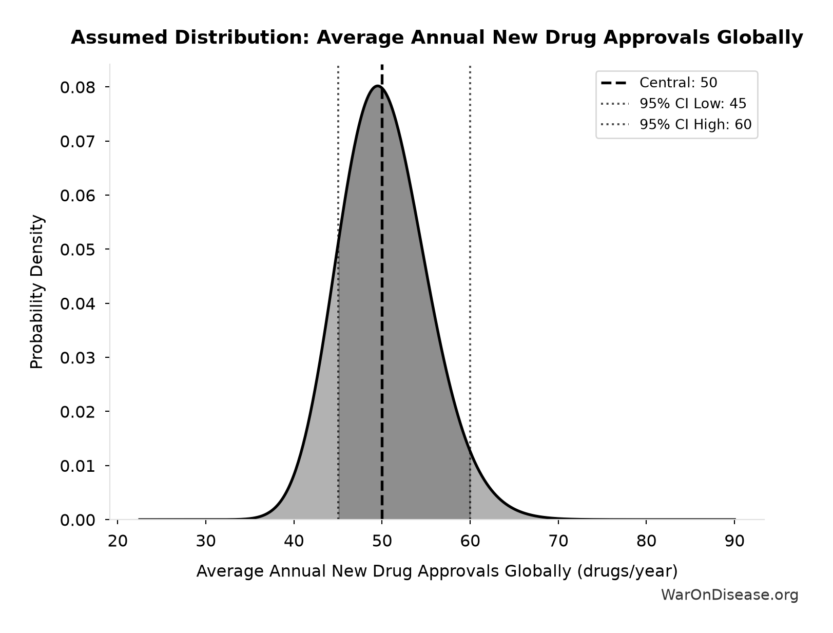
This chart shows the assumed probability distribution for this parameter. The shaded region represents the 95% confidence interval where we expect the true value to fall.
✓ High confidence
Current Global Clinical Trials per Year: 3,300 trials/year
Note📊 Details
Current global clinical trials per year
Source:23
Uncertainty Range
Technical: 95% CI: [2,640 trials/year, 3,960 trials/year] • Distribution: Lognormal
What this means: This estimate has moderate uncertainty. The true value likely falls between 2,640 trials/year and 3,960 trials/year (±20%). This represents a reasonable range that our Monte Carlo simulations account for when calculating overall uncertainty in the results.
The lognormal distribution means values can’t go negative and have a longer tail toward higher values (common for costs and populations).
Input Distribution
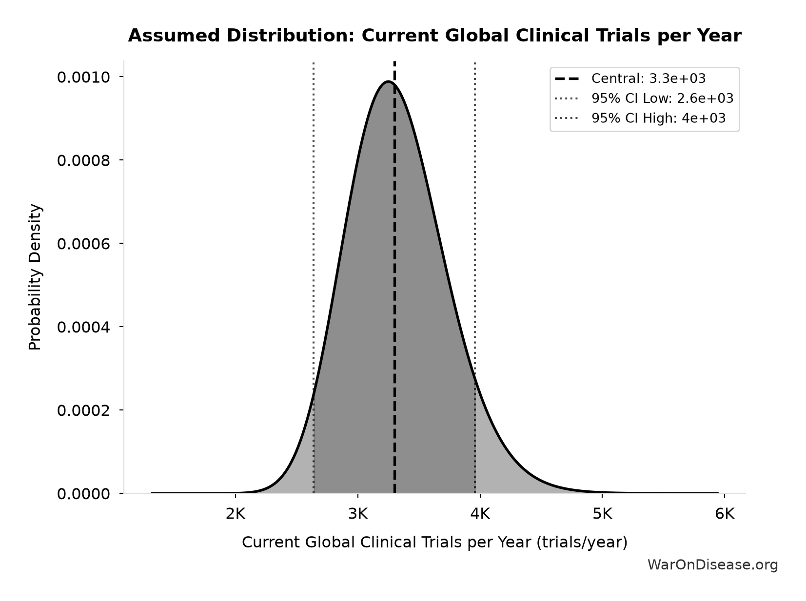
This chart shows the assumed probability distribution for this parameter. The shaded region represents the 95% confidence interval where we expect the true value to fall.
✓ High confidence
Annual Global Clinical Trial Participants: 1.9 million patients/year
Note📊 Details
Annual global clinical trial participants (IQVIA 2022: 1.9M post-COVID normalization)
Source:9
Uncertainty Range
Technical: 95% CI: [1.5 million patients/year, 2.3 million patients/year] • Distribution: Lognormal
What this means: This estimate has moderate uncertainty. The true value likely falls between 1.5 million patients/year and 2.3 million patients/year (±21%). This represents a reasonable range that our Monte Carlo simulations account for when calculating overall uncertainty in the results.
The lognormal distribution means values can’t go negative and have a longer tail toward higher values (common for costs and populations).
Input Distribution
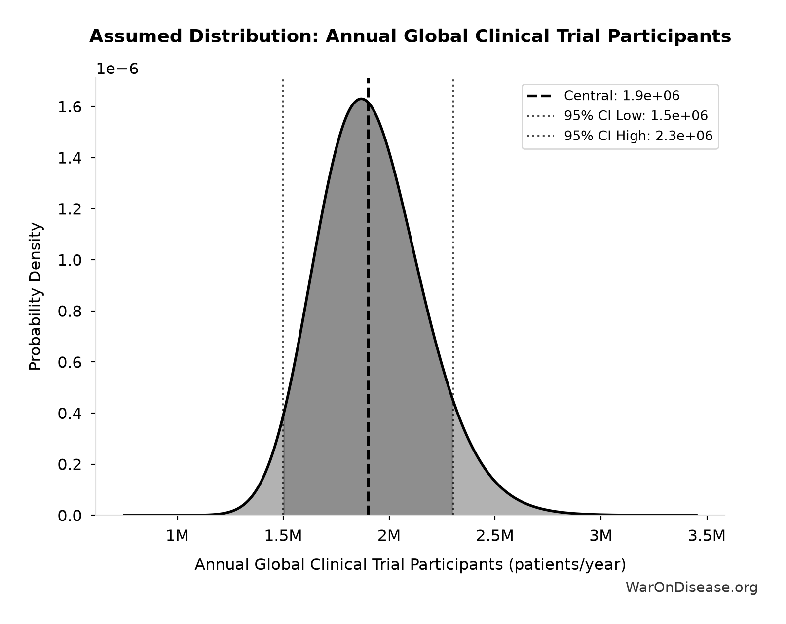
This chart shows the assumed probability distribution for this parameter. The shaded region represents the 95% confidence interval where we expect the true value to fall.
✓ High confidence
Pragmatic Trial Cost per Patient: $929
Note📊 Details
Embedded pragmatic trial cost per patient. Uses ADAPTABLE trial ($929) as DELIBERATELY CONSERVATIVE central estimate. Ramsberg & Platt (2018) reviewed 108 embedded pragmatic trials; 64 with cost data had median of only $97/patient - this estimate may overstate costs by 10x. Confidence interval spans meta-analysis median to complex chronic disease trials.
Source:1
Uncertainty Range
Technical: 95% CI: [$97, $3,000] • Distribution: Lognormal
What this means: This estimate is highly uncertain. The true value likely falls between $97 and $3,000 (±156%). This represents a very wide range that our Monte Carlo simulations account for when calculating overall uncertainty in the results.
The lognormal distribution means values can’t go negative and have a longer tail toward higher values (common for costs and populations).
Input Distribution
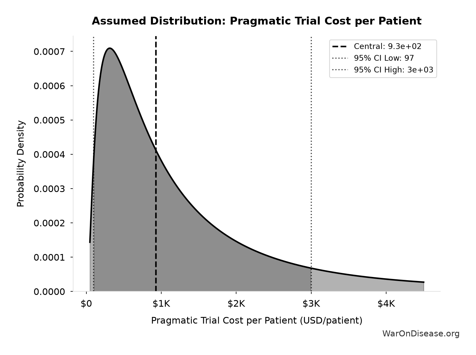
This chart shows the assumed probability distribution for this parameter. The shaded region represents the 95% confidence interval where we expect the true value to fall.
~ Medium confidence
Drug Development Cost (1980s): $194 million
Note📊 Details
Drug development cost in 1980s (compounded to approval, 1990 dollars)
Source:37
Uncertainty Range
Technical: 95% CI: [$146 million, $242 million] • Distribution: Lognormal
What this means: This estimate has moderate uncertainty. The true value likely falls between $146 million and $242 million (±25%). This represents a reasonable range that our Monte Carlo simulations account for when calculating overall uncertainty in the results.
The lognormal distribution means values can’t go negative and have a longer tail toward higher values (common for costs and populations).
Input Distribution
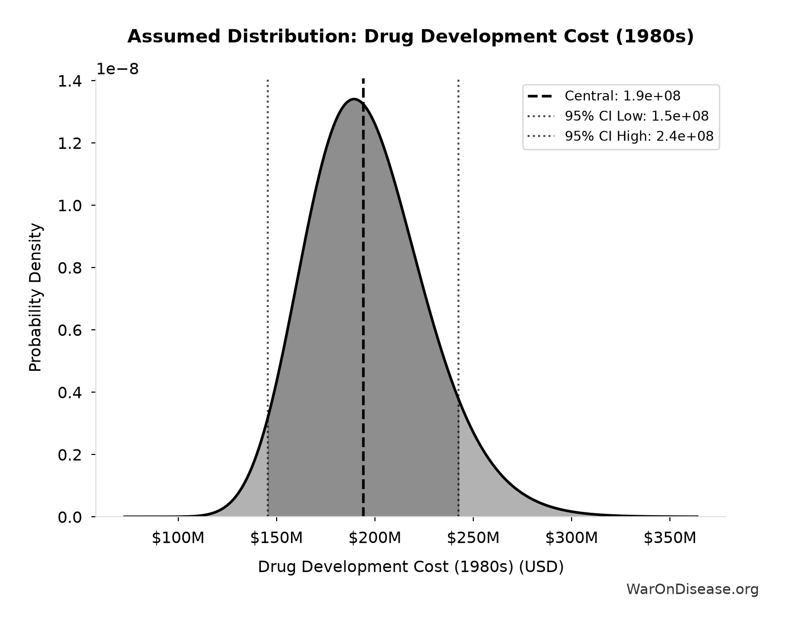
This chart shows the assumed probability distribution for this parameter. The shaded region represents the 95% confidence interval where we expect the true value to fall.
✓ High confidence
Drug Repurposing Success Rate: 30%
Note📊 Details
Percentage of drugs that gain at least one new indication after initial approval
Source:10
✓ High confidence
Regulatory Delay for Efficacy Testing Post-Safety Verification: 8.2 years
Note📊 Details
Regulatory delay for efficacy testing (Phase II/III) post-safety verification. Based on BIO 2021 industry survey. Note: This is for drugs that COMPLETE the pipeline - survivor bias means actual delay for any given disease may be longer if candidates fail and must restart.
Source:11
Uncertainty Range
Technical: Distribution: Normal (SE: 2 years)
Input Distribution
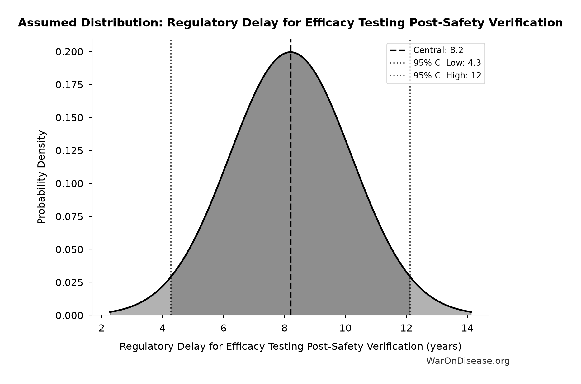
This chart shows the assumed probability distribution for this parameter. The shaded region represents the 95% confidence interval where we expect the true value to fall.
~ Medium confidence • 📊 Peer-reviewed • Updated 2021
FDA Phase 1 to Approval Timeline: 10.5 years
Note📊 Details
FDA timeline from Phase 1 start to approval. Derived from BIO 2021 industry survey: Phase 1 (2.3 years) + efficacy lag (8.2 years) = 10.5 years. Consistent with PMC meta-analysis finding 9.1 years median (95% CI: 8.2-10.0).
Source:11
Uncertainty Range
Technical: 95% CI: [6 years, 12 years] • Distribution: Gamma (SE: 2 years)
What this means: There’s significant uncertainty here. The true value likely falls between 6 years and 12 years (±29%). This represents a wide range that our Monte Carlo simulations account for when calculating overall uncertainty in the results.
The gamma distribution means values follow a specific statistical pattern.
Input Distribution
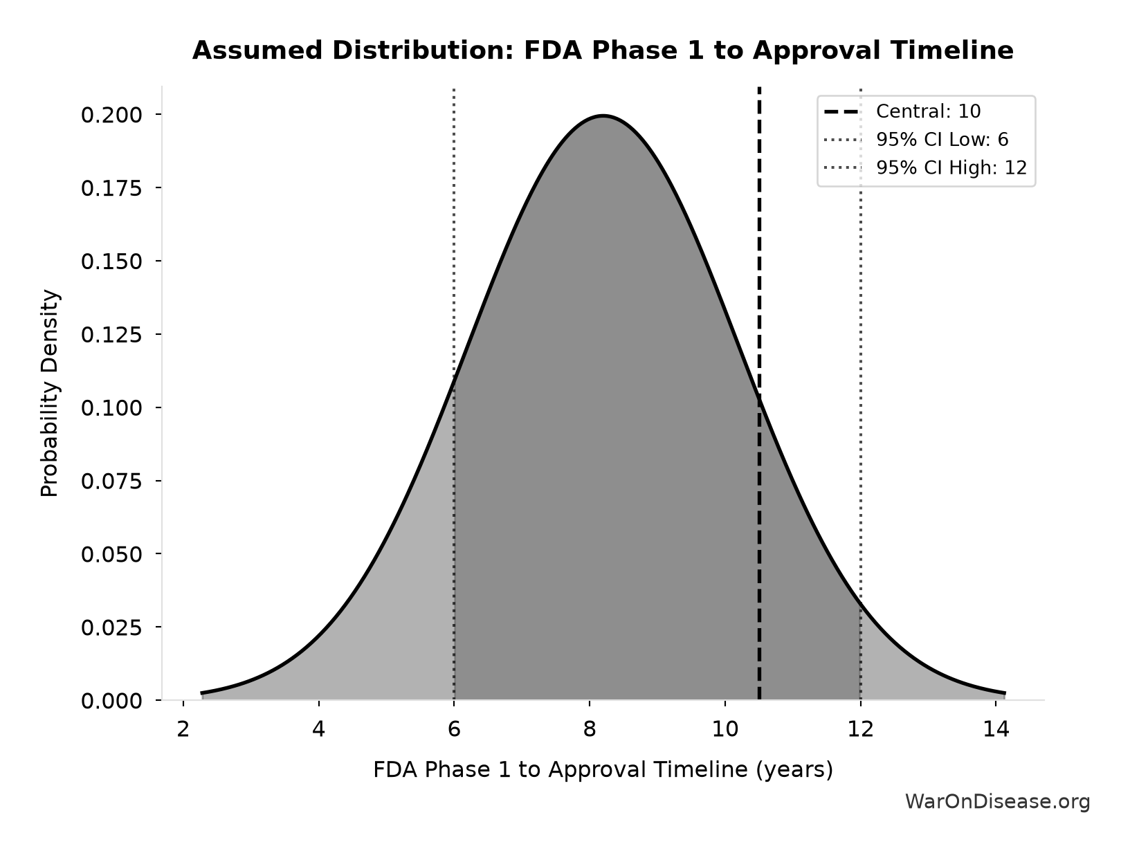
This chart shows the assumed probability distribution for this parameter. The shaded region represents the 95% confidence interval where we expect the true value to fall.
✓ High confidence
GiveWell Midpoint of Modeled Cost per Life Saved Range: $4,500
Note📊 Details
Midpoint of GiveWell’s cited $3,500 to $5,500 modeled cost-per-life-saved range across top charities
Source:3
Uncertainty Range
Technical: Distribution: Fixed
✓ High confidence
Global Annual DALY Burden: 2.88 billion DALYs/year
Note📊 Details
Global annual DALY burden from all diseases and injuries (WHO/IHME Global Burden of Disease 2021). Includes both YLL (years of life lost) and YLD (years lived with disability) from all causes.
Source:12
Uncertainty Range
Technical: Distribution: Normal (SE: 150 million DALYs/year)
Input Distribution
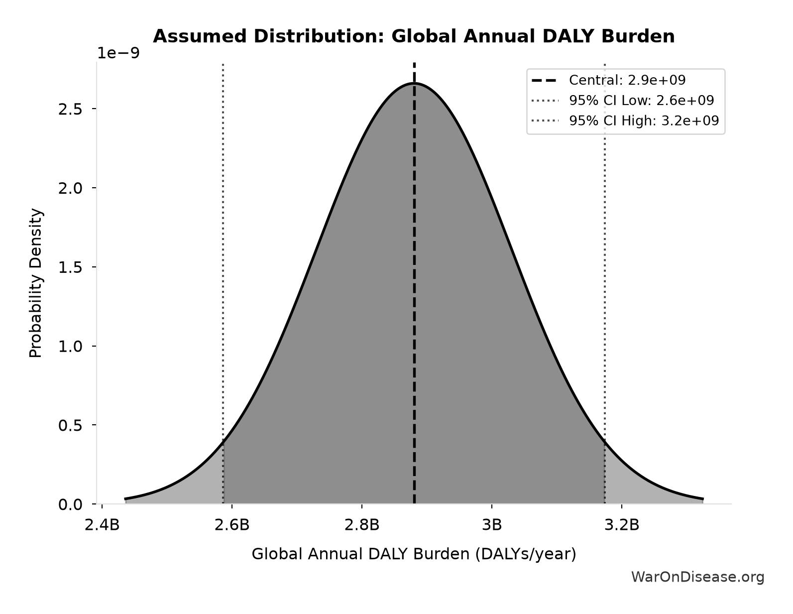
This chart shows the assumed probability distribution for this parameter. The shaded region represents the 95% confidence interval where we expect the true value to fall.
✓ High confidence • 📊 Peer-reviewed
Annual Deaths from All Diseases and Aging Globally: 55 million deaths/year
Note📊 Details
Annual deaths from all diseases and aging globally
Source:4
Uncertainty Range
Technical: Distribution: Normal (SE: 5 million deaths/year)
Input Distribution
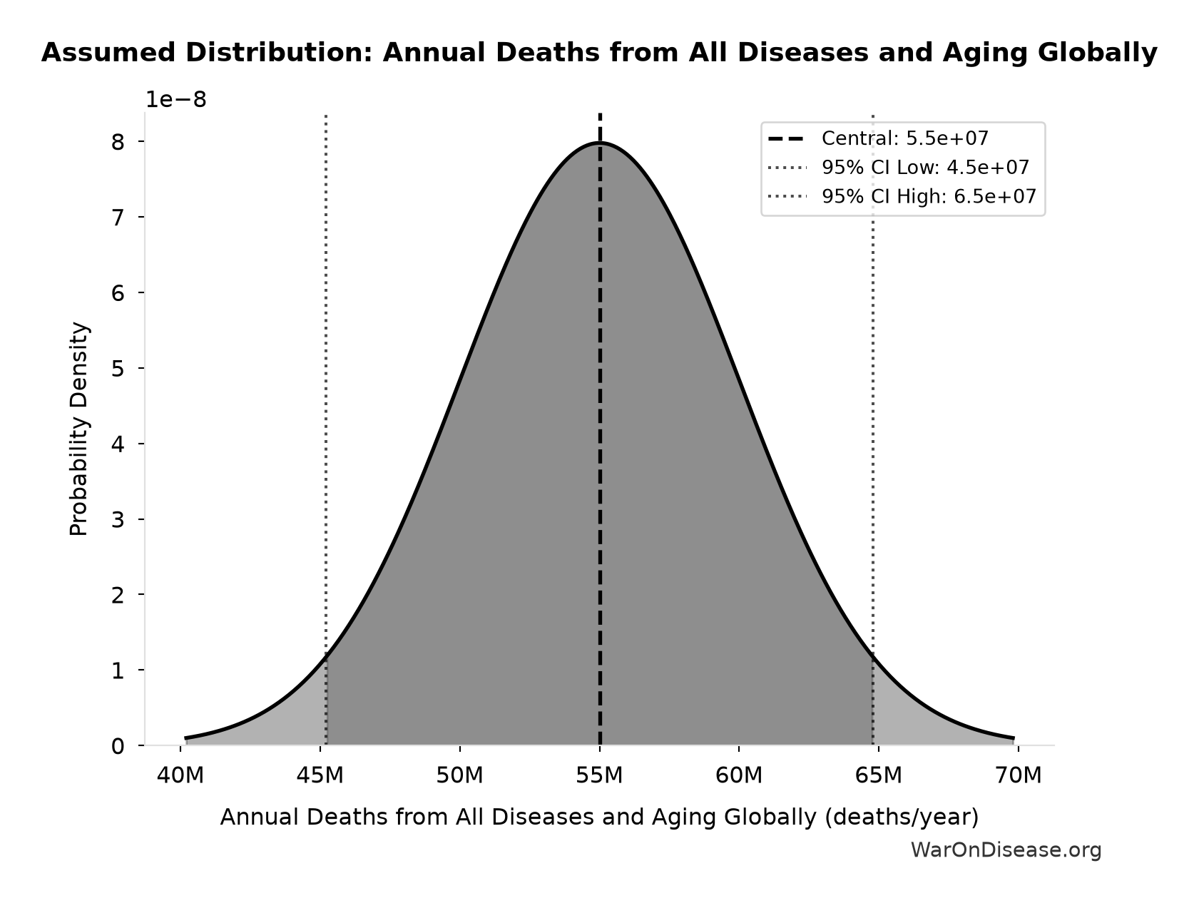
This chart shows the assumed probability distribution for this parameter. The shaded region represents the 95% confidence interval where we expect the true value to fall.
✓ High confidence
Annual Days of Chronic Disease Therapy: 1.28 trillion days
Note📊 Details
Annual days of therapy for chronic conditions globally (diabetes, CVD, respiratory, cancer). IQVIA reports 1.8 trillion total days of therapy in 2019, with 71% for chronic conditions.
Source:35
Uncertainty Range
Technical: 95% CI: [1 trillion days, 1.5 trillion days] • Distribution: Lognormal
What this means: This estimate has moderate uncertainty. The true value likely falls between 1 trillion days and 1.5 trillion days (±20%). This represents a reasonable range that our Monte Carlo simulations account for when calculating overall uncertainty in the results.
The lognormal distribution means values can’t go negative and have a longer tail toward higher values (common for costs and populations).
Input Distribution
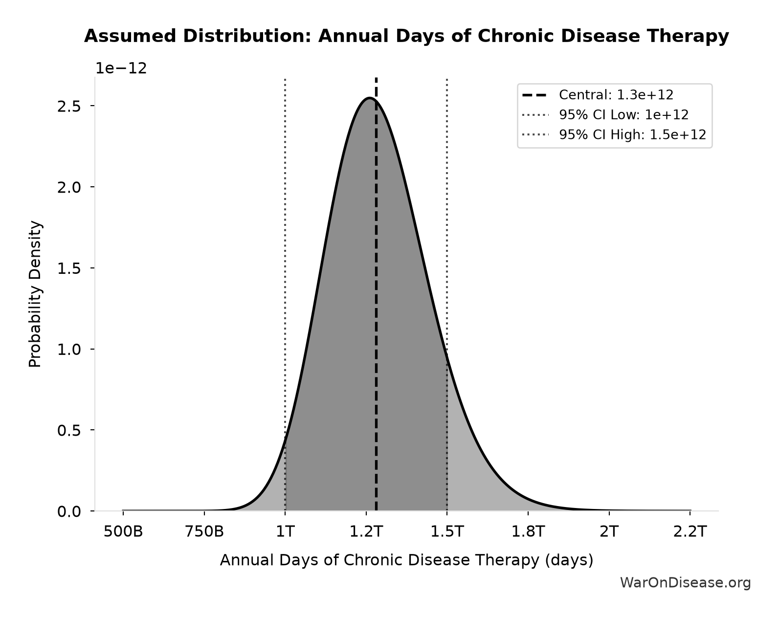
This chart shows the assumed probability distribution for this parameter. The shaded region represents the 95% confidence interval where we expect the true value to fall.
~ Medium confidence
Annual Global Spending on Clinical Trials: $60 billion
Note📊 Details
Annual global spending on clinical trials (Industry: $45-60B + Government: $3-6B + Nonprofits: $2-5B). Conservative estimate using 15-20% of $300B total pharma R&D, not inflated market size projections.
Source:13
Uncertainty Range
Technical: 95% CI: [$50 billion, $75 billion] • Distribution: Lognormal (SE: $10 billion)
What this means: This estimate has moderate uncertainty. The true value likely falls between $50 billion and $75 billion (±21%). This represents a reasonable range that our Monte Carlo simulations account for when calculating overall uncertainty in the results.
The lognormal distribution means values can’t go negative and have a longer tail toward higher values (common for costs and populations).
Input Distribution
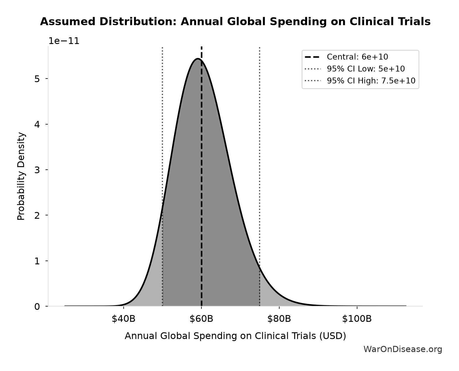
This chart shows the assumed probability distribution for this parameter. The shaded region represents the 95% confidence interval where we expect the true value to fall.
✓ High confidence
Global Daily Deaths from Disease and Aging: 150 thousand deaths/day
Note📊 Details
Total global deaths per day from all disease and aging (WHO Global Burden of Disease 2024)
Source:4
Uncertainty Range
Technical: Distribution: Normal (SE: 7,500 deaths/day)
Input Distribution
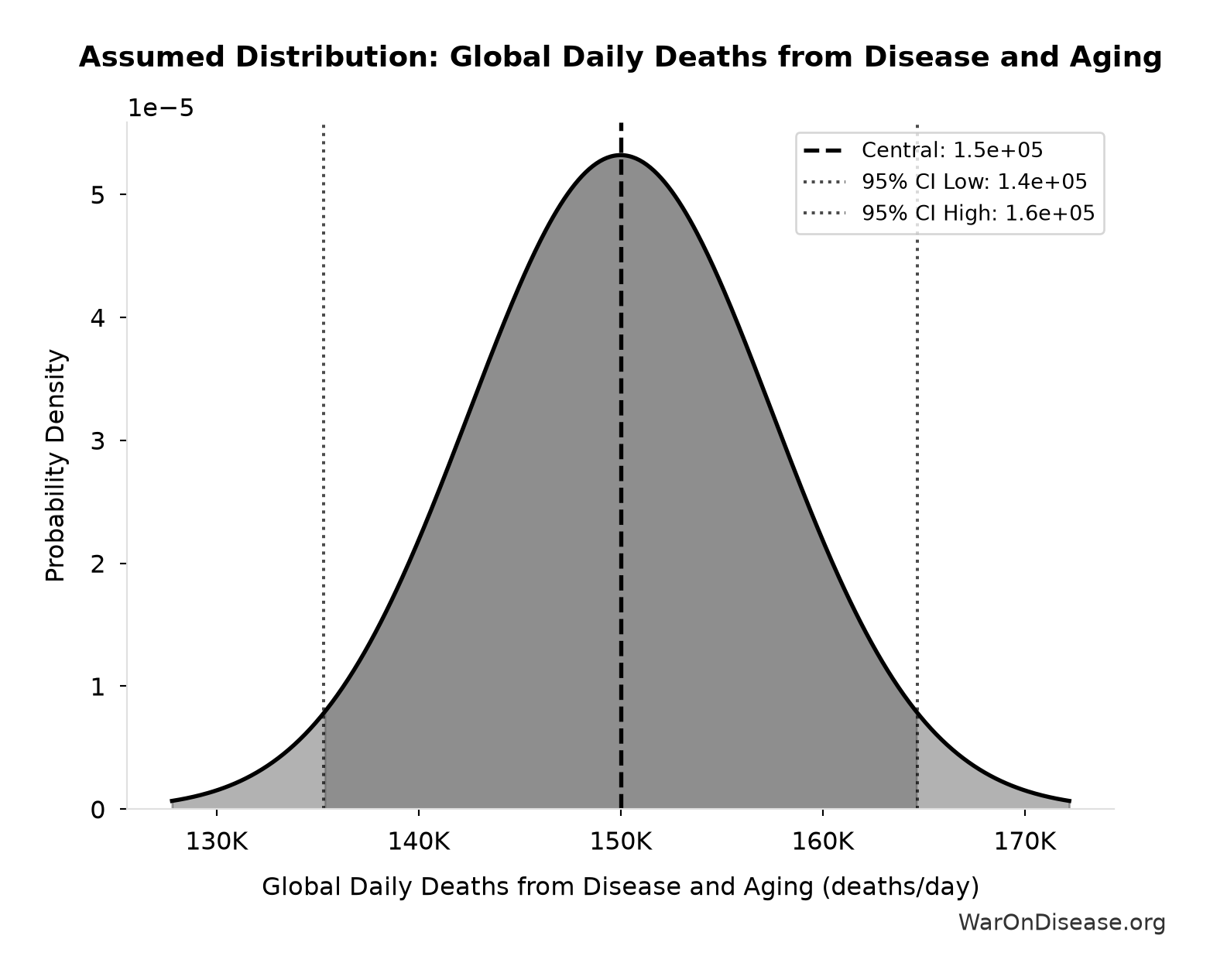
This chart shows the assumed probability distribution for this parameter. The shaded region represents the 95% confidence interval where we expect the true value to fall.
✓ High confidence • 📊 Peer-reviewed
Global GDP (2025): $115 trillion
Note📊 Details
Global nominal GDP (2025 estimate). From Political Dysfunction Tax paper citing StatisticsTimes/IMF World Economic Outlook. Used for calculating global opportunity costs as percentage of world economic output. Note: Latest IMF data shows $117T.
Source:14
Uncertainty Range
Technical: Distribution: Fixed
✓ High confidence
Remaining Life Expectancy at Age 60 (Global): 21 years
Note📊 Details
Additional years a person alive at age 60 can expect to live, global both-sexes (WHO life tables: 21.0 years in 2019; 19.6 in COVID-depressed 2021). This is CONDITIONAL remaining life expectancy, not life-expectancy-at-birth minus age: at-birth figures carry child mortality that someone who reached 60 already survived, so subtracting an age from them understates remaining years by roughly 40% at this age. Used for years-of-life-lost per efficacy-lag death. The GBD reference life table would give more (~23 years at 60); WHO period tables are the lower of the two standard choices.
Source:15
Uncertainty Range
Technical: 95% CI: [19.6 years, 22 years] • Distribution: Normal
What this means: We’re quite confident in this estimate. The true value likely falls between 19.6 years and 22 years (±6%). This represents a narrow range that our Monte Carlo simulations account for when calculating overall uncertainty in the results.
The normal distribution means values cluster around the center with equal chances of being higher or lower.
Input Distribution
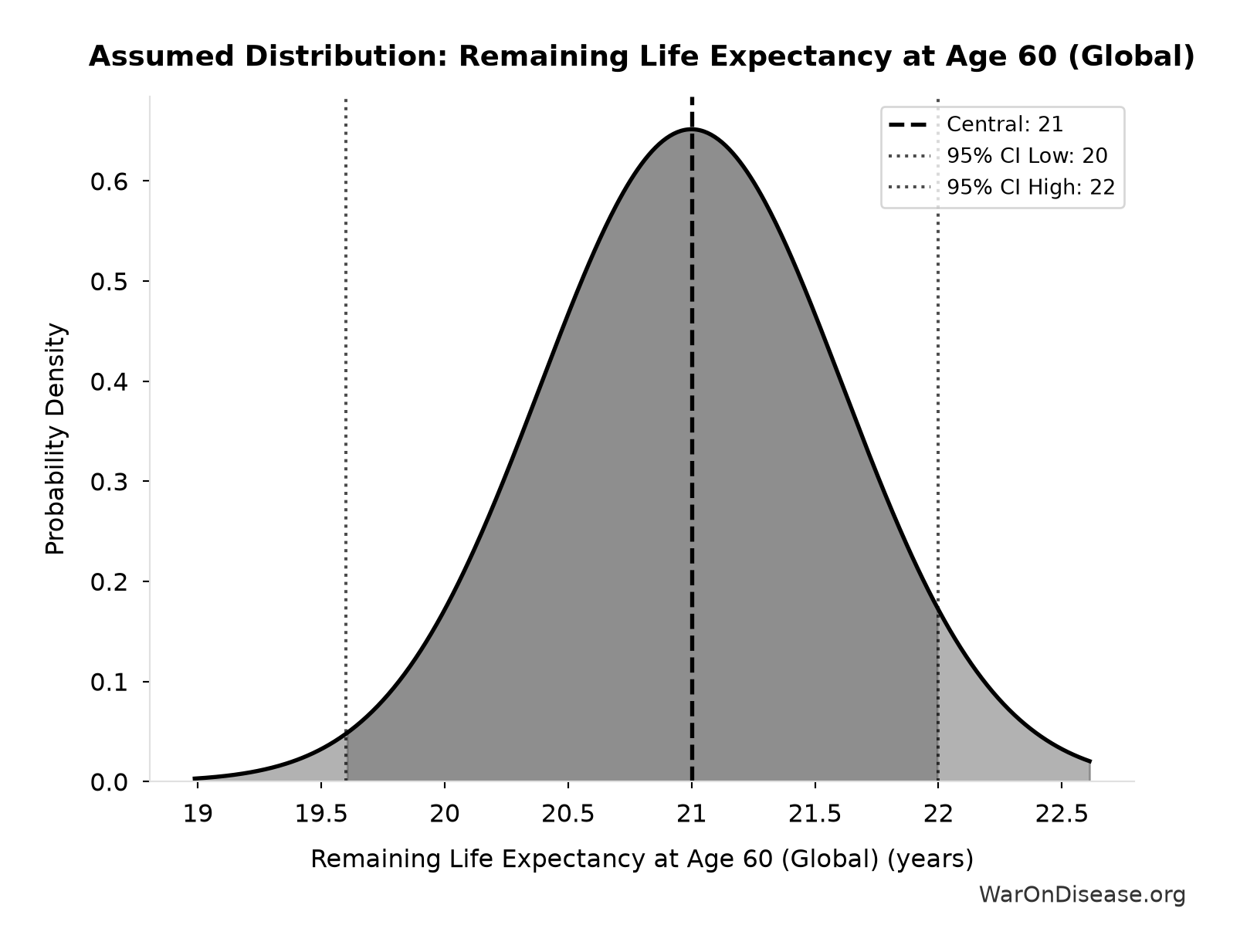
This chart shows the assumed probability distribution for this parameter. The shaded region represents the 95% confidence interval where we expect the true value to fall.
✓ High confidence
Global Military Spending in 2024: $2.72 trillion
Note📊 Details
Global military spending in 2024
Source:16
Uncertainty Range
Technical: Distribution: Fixed
✓ High confidence
YLD Proportion of Total DALYs: 0.39 proportion
Note📊 Details
Proportion of global DALYs that are YLD (years lived with disability) vs YLL (years of life lost). From GBD 2021: 1.13B YLD out of 2.88B total DALYs = 39%.
Source:12
Uncertainty Range
Technical: Distribution: Normal (SE: 0.03 proportion)
Input Distribution
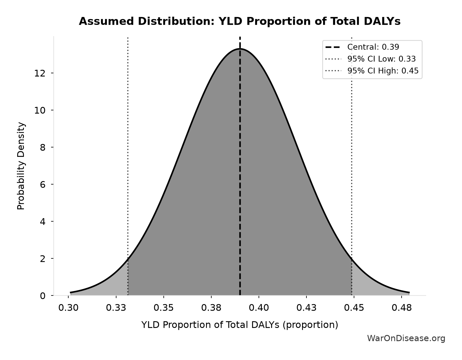
This chart shows the assumed probability distribution for this parameter. The shaded region represents the 95% confidence interval where we expect the true value to fall.
✓ High confidence • 📊 Peer-reviewed
Human Interactome Targeted by Drugs: 12%
Note📊 Details
Percentage of human interactome (protein-protein interactions) targeted by drugs
Source:17
✓ High confidence
Diseases Getting First Treatment Per Year: 15 diseases/year
Note📊 Details
Number of diseases that receive their FIRST effective treatment each year under current system. ~9 rare diseases/year (based on 40 years of ODA: 350 with treatment ÷ 40 years), plus ~5-10 common diseases. Note: FDA approves ~50 drugs/year, but most are for diseases that already have treatments.
Source:18
Uncertainty Range
Technical: 95% CI: [8 diseases/year, 30 diseases/year] • Distribution: Lognormal
What this means: This estimate is highly uncertain. The true value likely falls between 8 diseases/year and 30 diseases/year (±73%). This represents a very wide range that our Monte Carlo simulations account for when calculating overall uncertainty in the results.
The lognormal distribution means values can’t go negative and have a longer tail toward higher values (common for costs and populations).
Input Distribution
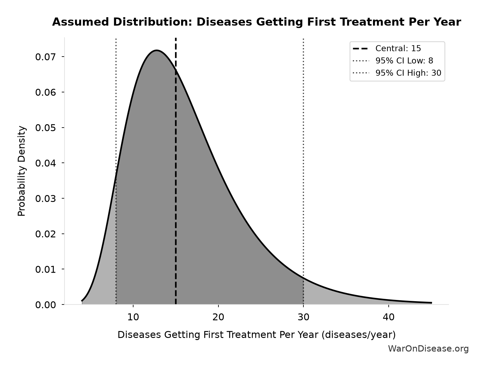
This chart shows the assumed probability distribution for this parameter. The shaded region represents the 95% confidence interval where we expect the true value to fall.
? Low confidence
NIH Standard Research Cost per QALY: $50,000
Note📊 Details
Typical cost per QALY for standard NIH-funded medical research portfolio. Reflects the inefficiency of traditional RCTs and basic research-heavy allocation. See confidence_interval for range; ICER uses higher thresholds for value-based pricing.
Source:19
Uncertainty Range
Technical: 95% CI: [$20,000, $100,000] • Distribution: Lognormal
What this means: This estimate is highly uncertain. The true value likely falls between $20,000 and $100,000 (±80%). This represents a very wide range that our Monte Carlo simulations account for when calculating overall uncertainty in the results.
The lognormal distribution means values can’t go negative and have a longer tail toward higher values (common for costs and populations).
Input Distribution
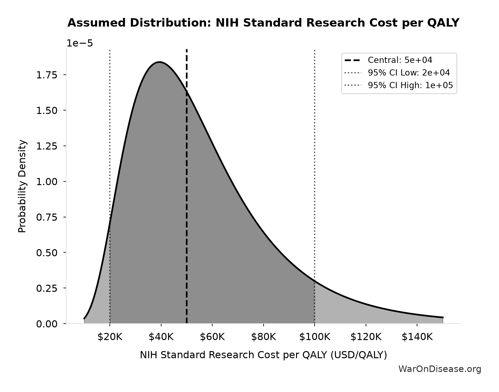
This chart shows the assumed probability distribution for this parameter. The shaded region represents the 95% confidence interval where we expect the true value to fall.
~ Medium confidence
Pharma Drug Development Cost (Current System): $2.6 billion
Note📊 Details
Average cost to develop one drug in current system
Source:20
Uncertainty Range
Technical: 95% CI: [$1.5 billion, $4 billion] • Distribution: Lognormal (SE: $500 million)
What this means: There’s significant uncertainty here. The true value likely falls between $1.5 billion and $4 billion (±48%). This represents a wide range that our Monte Carlo simulations account for when calculating overall uncertainty in the results.
The lognormal distribution means values can’t go negative and have a longer tail toward higher values (common for costs and populations).
Input Distribution
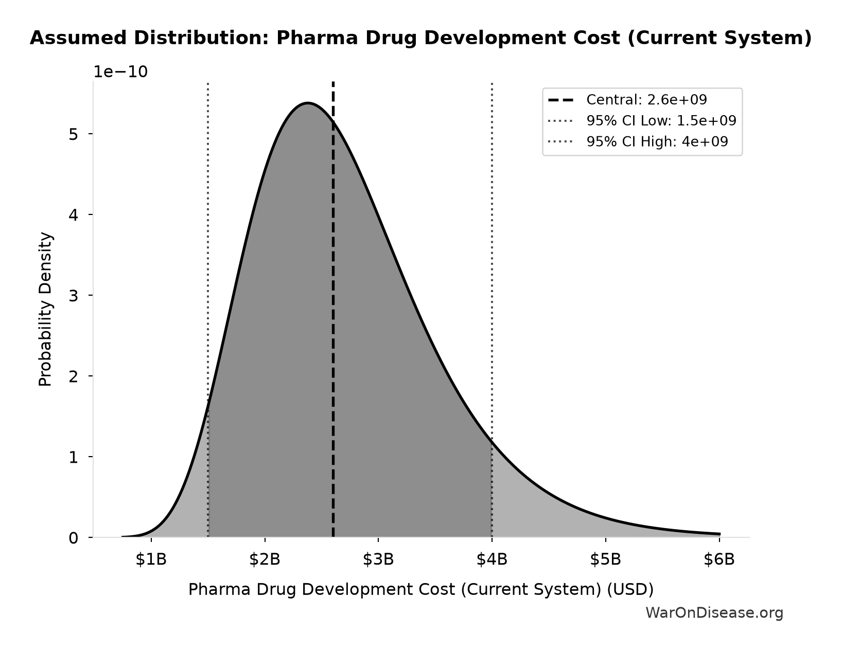
This chart shows the assumed probability distribution for this parameter. The shaded region represents the 95% confidence interval where we expect the true value to fall.
✓ High confidence • 📊 Peer-reviewed
Annual Life-Years Saved by Pharmaceuticals: 149 million life-years
Note📊 Details
Annual life-years saved by pharmaceutical innovations globally. Lichtenberg (2019, NBER WP 25483) found that drugs launched after 1981 saved 148.7M life-years in 2013 across 22 countries using 3-way fixed-effects regression (disease-country-year). 95% CI [79.4M, 239.8M] propagated from Table 2 regression standard errors (β₀₋₁₁=-0.031±0.008, β₁₂₊=-0.057±0.013).
Source:21
Uncertainty Range
Technical: 95% CI: [79.4 million life-years, 240 million life-years] • Distribution: Lognormal
What this means: This estimate is highly uncertain. The true value likely falls between 79.4 million life-years and 240 million life-years (±54%). This represents a very wide range that our Monte Carlo simulations account for when calculating overall uncertainty in the results.
The lognormal distribution means values can’t go negative and have a longer tail toward higher values (common for costs and populations).
Input Distribution
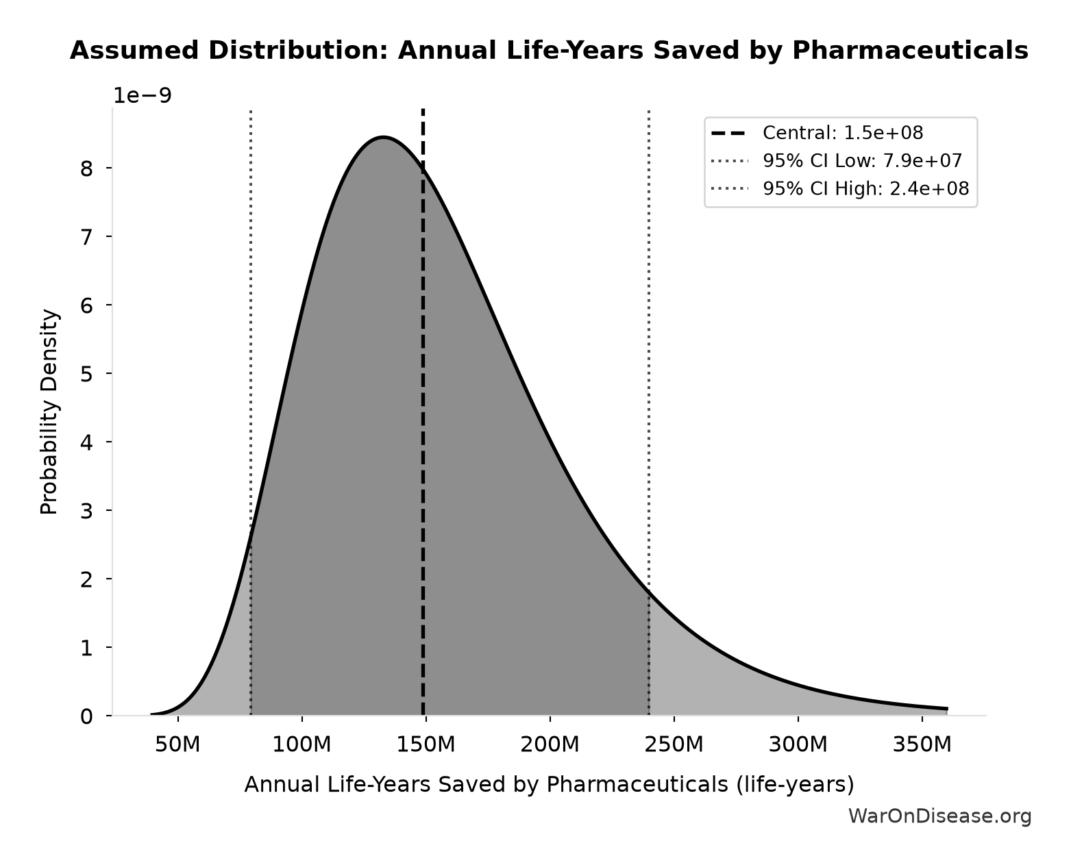
This chart shows the assumed probability distribution for this parameter. The shaded region represents the 95% confidence interval where we expect the true value to fall.
~ Medium confidence
Pharma Drug Success Rate (Current System): 10%
Note📊 Details
Percentage of drugs that reach market in current system
Source:22
✓ High confidence • 📊 Peer-reviewed
Phase I Safety Trial Duration: 2.3 years
Note📊 Details
Phase 2/3 Share of Clinical Trial Costs: 69%
Note📊 Details
Percentage of total clinical trial spending on Phase 2/3 efficacy testing (Phase 2: 24% + Phase 3: 45%)
Source:23
Uncertainty Range
Technical: Distribution: Normal (SE: 5%)
Input Distribution
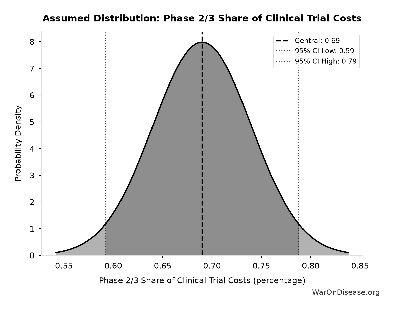
This chart shows the assumed probability distribution for this parameter. The shaded region represents the 95% confidence interval where we expect the true value to fall.
✓ High confidence
Phase 3 Trial Total Cost (Minimum): $20 million
Note📊 Details
Pragmatic Trial Median Cost per Patient (PMC Review): $97
Note📊 Details
Median cost per patient in embedded pragmatic clinical trials (Ramsberg & Platt 2018: 108 trials reviewed, 64 with cost data). IQR: $19-$478 (2015 USD).
Source:25
Uncertainty Range
Technical: 95% CI: [$19, $478] • Distribution: Lognormal
What this means: This estimate is highly uncertain. The true value likely falls between $19 and $478 (±237%). This represents a very wide range that our Monte Carlo simulations account for when calculating overall uncertainty in the results.
The lognormal distribution means values can’t go negative and have a longer tail toward higher values (common for costs and populations).
Input Distribution
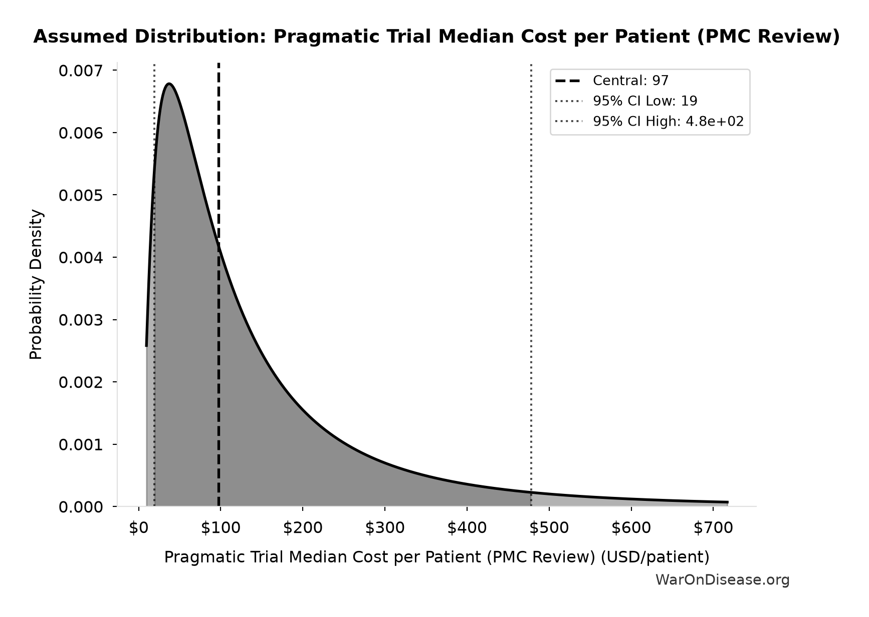
This chart shows the assumed probability distribution for this parameter. The shaded region represents the 95% confidence interval where we expect the true value to fall.
✓ High confidence
Post-1962 Drug Approval Reduction: 70%
Note📊 Details
Reduction in new drug approvals after 1962 Kefauver-Harris Amendment (70% drop from 43→17 drugs/year)
Source:26
✓ High confidence • Updated 1962-1970
Pre-1962 Drug Development Cost (1980 Dollars): $6.5 million
Note📊 Details
Average drug development cost before 1962 FDA efficacy regulations, adjusted to 1980 dollars (Baily 1972)
Source:27
Uncertainty Range
Technical: 95% CI: [$5.2 million, $7.8 million] • Distribution: Lognormal
What this means: This estimate has moderate uncertainty. The true value likely falls between $5.2 million and $7.8 million (±20%). This represents a reasonable range that our Monte Carlo simulations account for when calculating overall uncertainty in the results.
The lognormal distribution means values can’t go negative and have a longer tail toward higher values (common for costs and populations).
Input Distribution
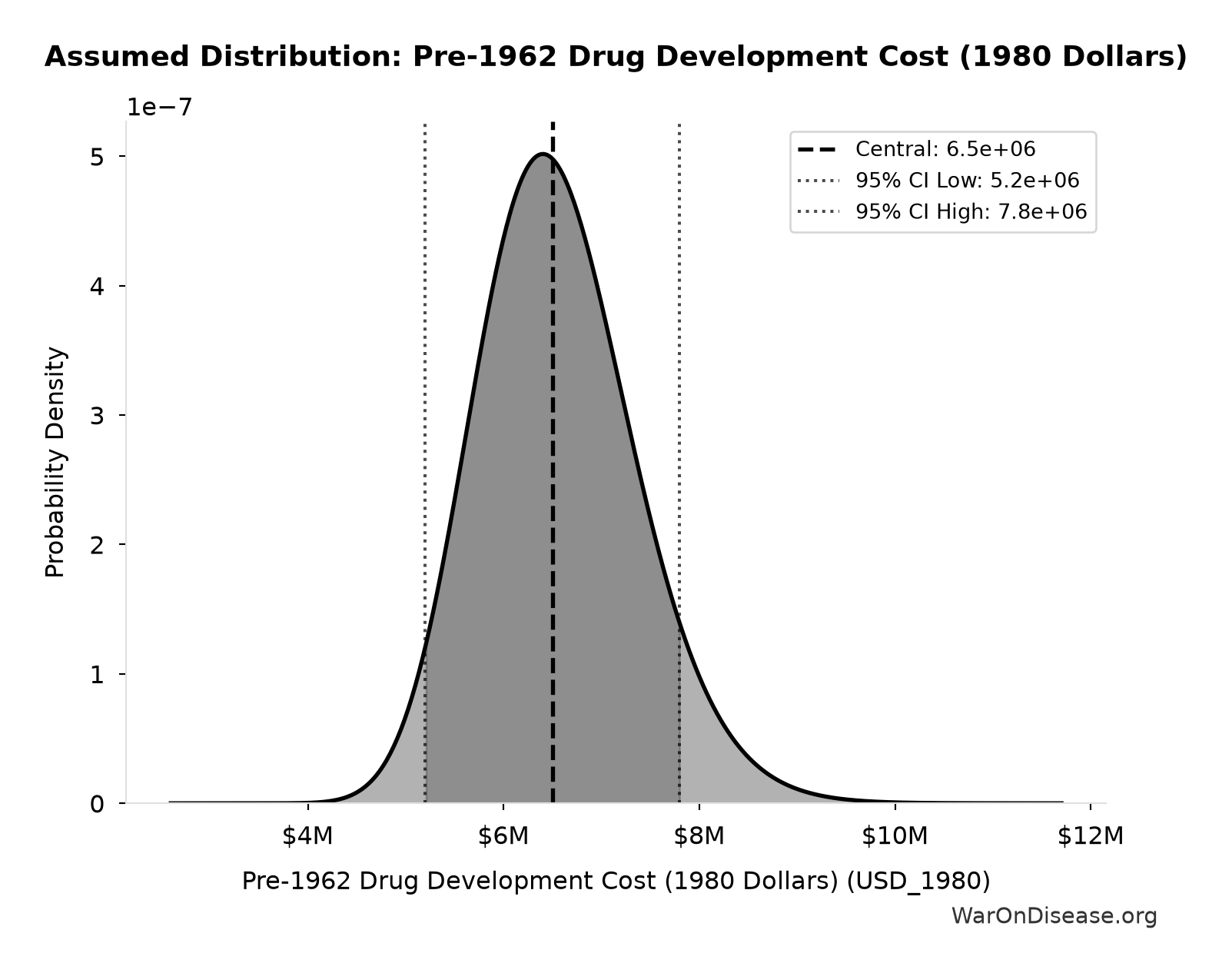
This chart shows the assumed probability distribution for this parameter. The shaded region represents the 95% confidence interval where we expect the true value to fall.
✓ High confidence • 📊 Peer-reviewed
Pre-1962 Drug Development Cost (2024 Dollars): $24.7 million
Note📊 Details
Pre-1962 drug development cost adjusted to 2024 dollars ($6.5M × 3.80 = $24.7M, CPI-adjusted from Baily 1972)
Source:27
Uncertainty Range
Technical: 95% CI: [$19.5 million, $30 million] • Distribution: Lognormal
What this means: This estimate has moderate uncertainty. The true value likely falls between $19.5 million and $30 million (±21%). This represents a reasonable range that our Monte Carlo simulations account for when calculating overall uncertainty in the results.
The lognormal distribution means values can’t go negative and have a longer tail toward higher values (common for costs and populations).
Input Distribution
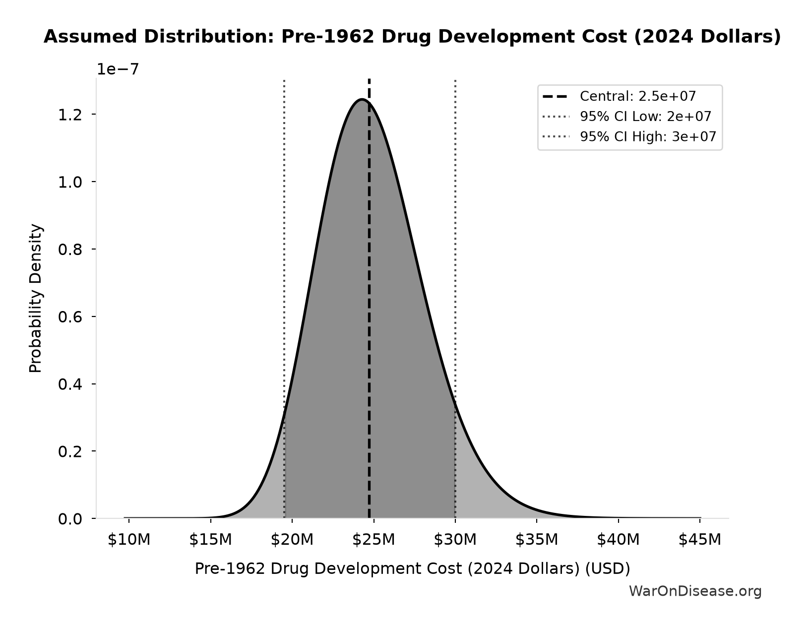
This chart shows the assumed probability distribution for this parameter. The shaded region represents the 95% confidence interval where we expect the true value to fall.
✓ High confidence • 📊 Peer-reviewed
Pre-1962 Physician Count (Unverified): 144 thousand physicians
Note📊 Details
Estimated physicians conducting real-world efficacy trials pre-1962 (unverified estimate)
Source:28
? Low confidence
Total Number of Rare Diseases Globally: 7,000 diseases
Note📊 Details
Total number of rare diseases globally
Source:39
Uncertainty Range
Technical: 95% CI: [6,000 diseases, 10,000 diseases] • Distribution: Normal
What this means: There’s significant uncertainty here. The true value likely falls between 6,000 diseases and 10,000 diseases (±29%). This represents a wide range that our Monte Carlo simulations account for when calculating overall uncertainty in the results.
The normal distribution means values cluster around the center with equal chances of being higher or lower.
Input Distribution
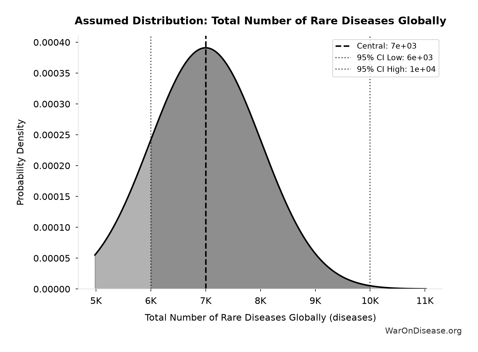
This chart shows the assumed probability distribution for this parameter. The shaded region represents the 95% confidence interval where we expect the true value to fall.
✓ High confidence
Recovery Trial Cost per Patient: $500
Note📊 Details
RECOVERY trial cost per patient. Note: RECOVERY was an outlier - hospital-based during COVID emergency, minimal extra procedures, existing NHS infrastructure, streamlined consent. Replicating this globally will be harder.
Source:29
Uncertainty Range
Technical: 95% CI: [$400, $2,500] • Distribution: Lognormal
What this means: This estimate is highly uncertain. The true value likely falls between $400 and $2,500 (±210%). This represents a very wide range that our Monte Carlo simulations account for when calculating overall uncertainty in the results.
The lognormal distribution means values can’t go negative and have a longer tail toward higher values (common for costs and populations).
Input Distribution
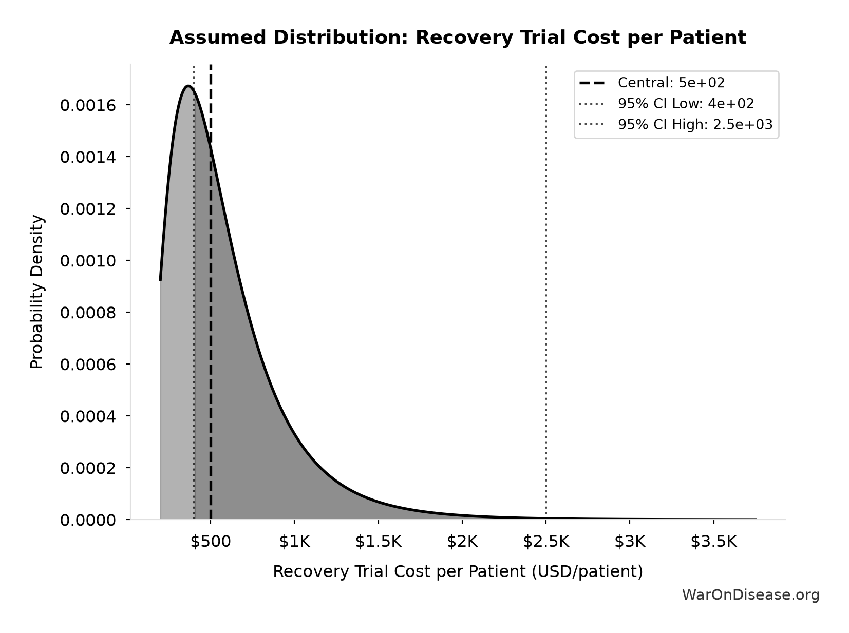
This chart shows the assumed probability distribution for this parameter. The shaded region represents the 95% confidence interval where we expect the true value to fall.
✓ High confidence
RECOVERY Trial Global Lives Saved: 1 million lives
Note📊 Details
Estimated lives saved globally by RECOVERY trial’s dexamethasone discovery. NHS England estimate (March 2021). Based on Águas et al. Nature Communications 2021 methodology applying RECOVERY trial mortality reductions (36% ventilated, 18% oxygen) to global COVID hospitalizations. Wide uncertainty range reflects extrapolation assumptions.
Source:30
Uncertainty Range
Technical: 95% CI: [500 thousand lives, 2 million lives] • Distribution: Lognormal
What this means: This estimate is highly uncertain. The true value likely falls between 500 thousand lives and 2 million lives (±75%). This represents a very wide range that our Monte Carlo simulations account for when calculating overall uncertainty in the results.
The lognormal distribution means values can’t go negative and have a longer tail toward higher values (common for costs and populations).
Input Distribution
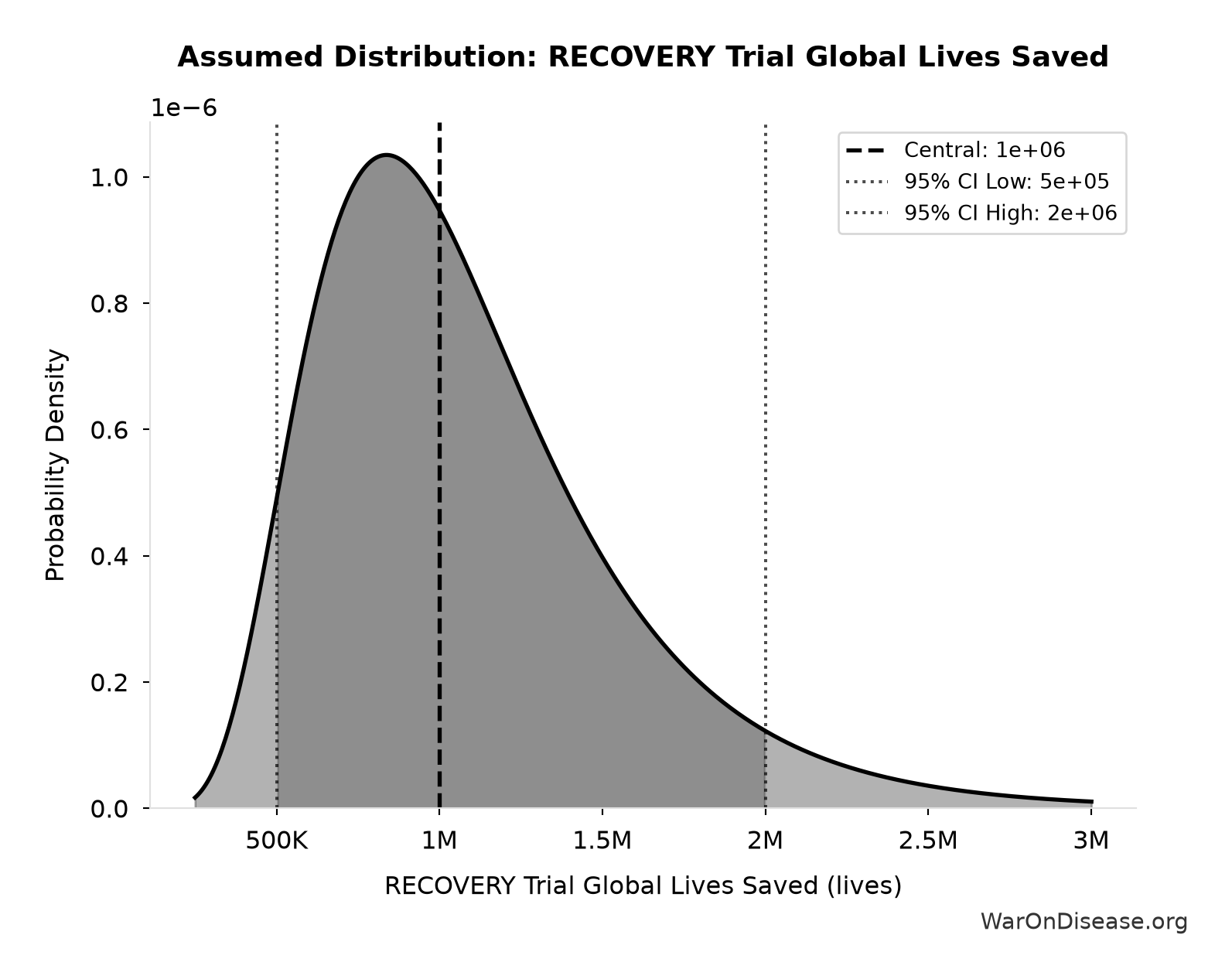
This chart shows the assumed probability distribution for this parameter. The shaded region represents the 95% confidence interval where we expect the true value to fall.
~ Medium confidence
RECOVERY Trial Total Cost: $20 million
Note📊 Details
Total cost of UK RECOVERY trial. Enrolled tens of thousands of patients across multiple treatment arms. Discovered dexamethasone reduces COVID mortality by ~1/3 in severe cases.
Source:31
Uncertainty Range
Technical: 95% CI: [$15 million, $25 million] • Distribution: Lognormal
What this means: This estimate has moderate uncertainty. The true value likely falls between $15 million and $25 million (±25%). This represents a reasonable range that our Monte Carlo simulations account for when calculating overall uncertainty in the results.
The lognormal distribution means values can’t go negative and have a longer tail toward higher values (common for costs and populations).
Input Distribution
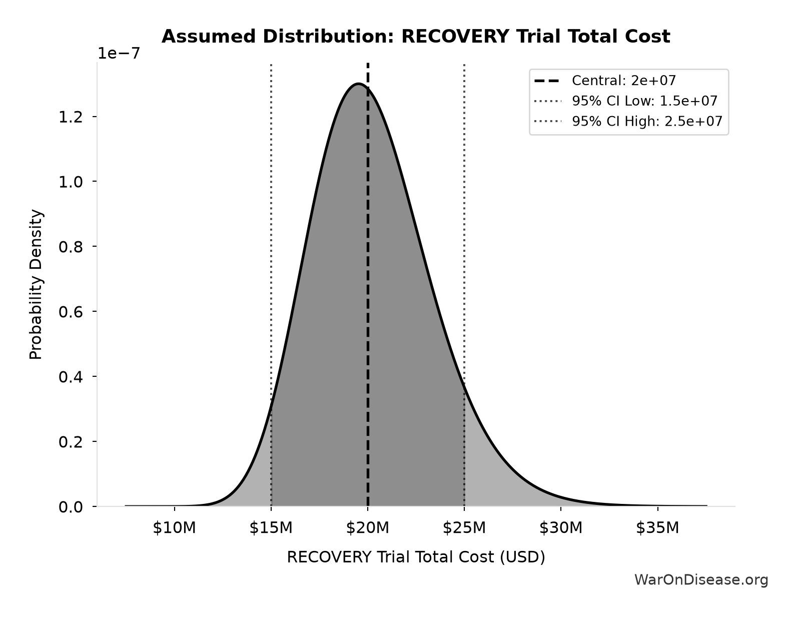
This chart shows the assumed probability distribution for this parameter. The shaded region represents the 95% confidence interval where we expect the true value to fall.
✓ High confidence
Mean Age of Preventable Death from Post-Safety Efficacy Delay: 62 years
Note📊 Details
Mean age of preventable death from post-safety efficacy testing regulatory delay (Phase 2-4)
Source:4
Uncertainty Range
Technical: Distribution: Normal (SE: 3 years)
Input Distribution
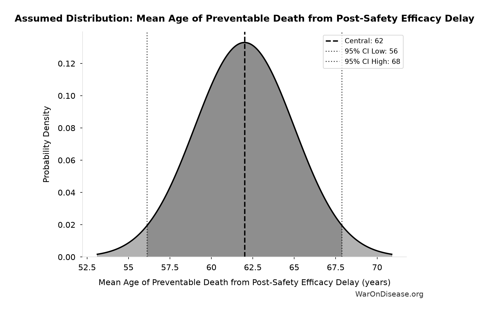
This chart shows the assumed probability distribution for this parameter. The shaded region represents the 95% confidence interval where we expect the true value to fall.
~ Medium confidence • 📊 Peer-reviewed
Pre-Death Suffering Period During Post-Safety Efficacy Delay: 6 years
Note📊 Details
Pre-death suffering period during post-safety efficacy testing delay (average years lived with untreated condition while awaiting Phase 2-4 completion)
Source:4
Uncertainty Range
Technical: 95% CI: [4 years, 9 years] • Distribution: Lognormal
What this means: There’s significant uncertainty here. The true value likely falls between 4 years and 9 years (±42%). This represents a wide range that our Monte Carlo simulations account for when calculating overall uncertainty in the results.
The lognormal distribution means values can’t go negative and have a longer tail toward higher values (common for costs and populations).
Input Distribution
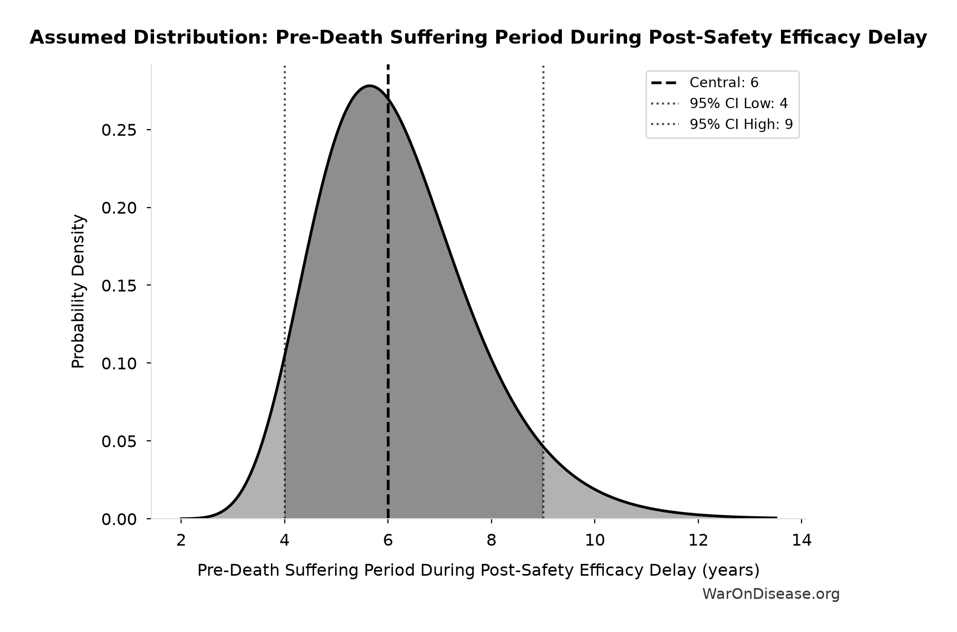
This chart shows the assumed probability distribution for this parameter. The shaded region represents the 95% confidence interval where we expect the true value to fall.
~ Medium confidence • 📊 Peer-reviewed
September 11 Deaths: 2,977 people
Note📊 Details
Total deaths in the September 11, 2001 attacks. 2,977 victims (excluding 19 hijackers). Used as a reference point for scale comparisons.
Source:40
Uncertainty Range
Technical: Distribution: Fixed
✓ High confidence
Standard Economic Value per QALY: $150,000
Note📊 Details
Standard economic value per QALY
Source:32
Uncertainty Range
Technical: Distribution: Normal (SE: $30,000)
Input Distribution
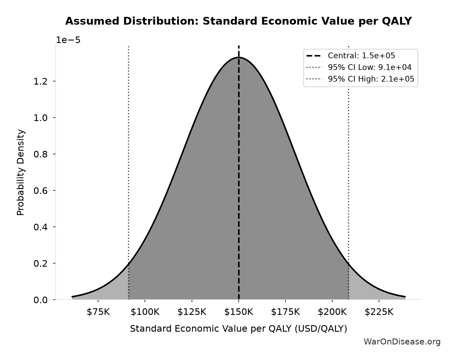
This chart shows the assumed probability distribution for this parameter. The shaded region represents the 95% confidence interval where we expect the true value to fall.
✓ High confidence
Thalidomide Cases Worldwide: 15,000 cases
Note📊 Details
Total thalidomide birth defect cases worldwide (1957-1962)
Source:41
Uncertainty Range
Technical: 95% CI: [10,000 cases, 20,000 cases] • Distribution: Lognormal
What this means: There’s significant uncertainty here. The true value likely falls between 10,000 cases and 20,000 cases (±33%). This represents a wide range that our Monte Carlo simulations account for when calculating overall uncertainty in the results.
The lognormal distribution means values can’t go negative and have a longer tail toward higher values (common for costs and populations).
Input Distribution
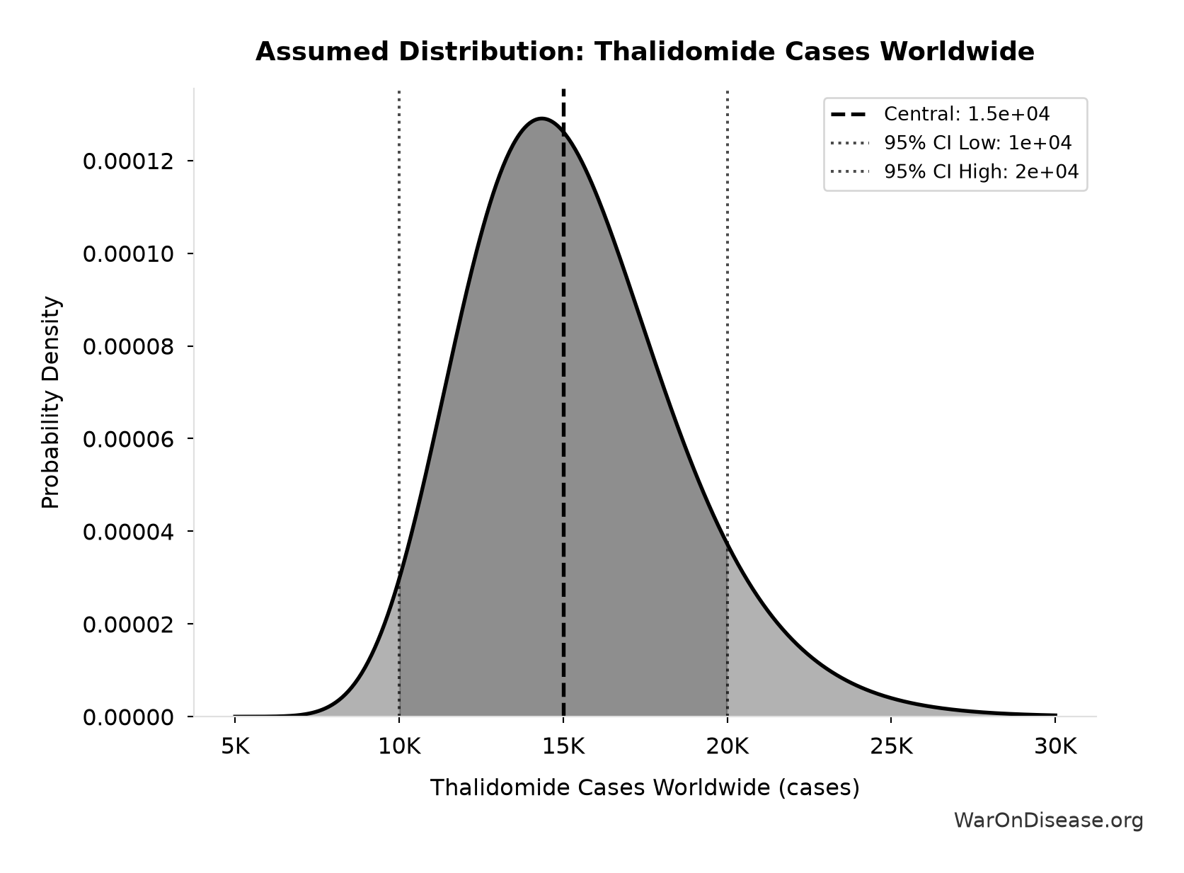
This chart shows the assumed probability distribution for this parameter. The shaded region represents the 95% confidence interval where we expect the true value to fall.
~ Medium confidence
Thalidomide Disability Weight: 0.4:1
Note📊 Details
Disability weight for thalidomide survivors (limb deformities, organ damage)
Source:42
Uncertainty Range
Technical: 95% CI: [0.32:1, 0.48:1] • Distribution: Lognormal
What this means: This estimate has moderate uncertainty. The true value likely falls between 0.32:1 and 0.48:1 (±20%). This represents a reasonable range that our Monte Carlo simulations account for when calculating overall uncertainty in the results.
The lognormal distribution means values can’t go negative and have a longer tail toward higher values (common for costs and populations).
Input Distribution
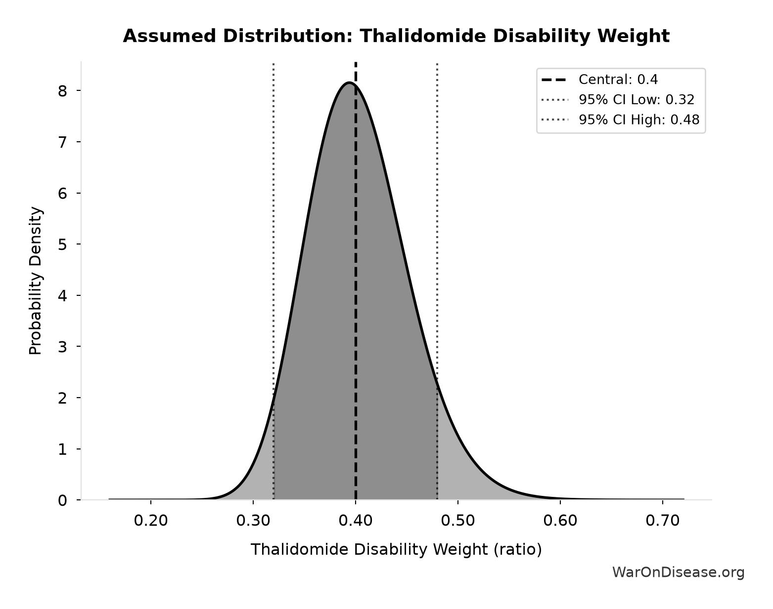
This chart shows the assumed probability distribution for this parameter. The shaded region represents the 95% confidence interval where we expect the true value to fall.
~ Medium confidence
Thalidomide Mortality Rate: 40%
Note📊 Details
Mortality rate for thalidomide-affected infants (died within first year)
Source:41
Uncertainty Range
Technical: 95% CI: [35%, 45%] • Distribution: Lognormal
What this means: This estimate has moderate uncertainty. The true value likely falls between 35% and 45% (±13%). This represents a reasonable range that our Monte Carlo simulations account for when calculating overall uncertainty in the results.
The lognormal distribution means values can’t go negative and have a longer tail toward higher values (common for costs and populations).
Input Distribution
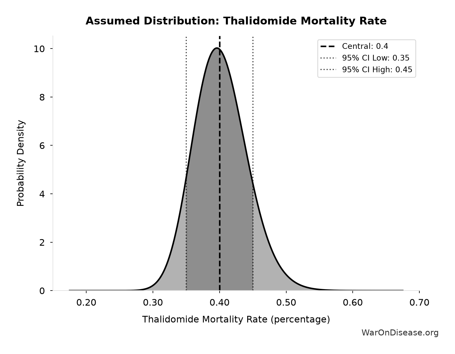
This chart shows the assumed probability distribution for this parameter. The shaded region represents the 95% confidence interval where we expect the true value to fall.
✓ High confidence
Thalidomide Survivor Lifespan: 60 years
Note📊 Details
Average lifespan for thalidomide survivors
Source:42
Uncertainty Range
Technical: 95% CI: [50 years, 70 years] • Distribution: Lognormal
What this means: This estimate has moderate uncertainty. The true value likely falls between 50 years and 70 years (±17%). This represents a reasonable range that our Monte Carlo simulations account for when calculating overall uncertainty in the results.
The lognormal distribution means values can’t go negative and have a longer tail toward higher values (common for costs and populations).
Input Distribution
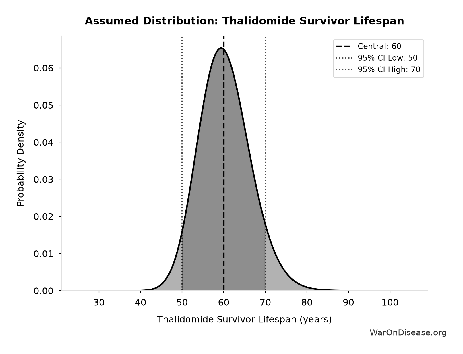
This chart shows the assumed probability distribution for this parameter. The shaded region represents the 95% confidence interval where we expect the true value to fall.
~ Medium confidence
US Population Share 1960: 6%
Note📊 Details
US share of world population in 1960
Source:43
Uncertainty Range
Technical: 95% CI: [5.5%, 6.5%] • Distribution: Lognormal
What this means: We’re quite confident in this estimate. The true value likely falls between 5.5% and 6.5% (±8%). This represents a narrow range that our Monte Carlo simulations account for when calculating overall uncertainty in the results.
The lognormal distribution means values can’t go negative and have a longer tail toward higher values (common for costs and populations).
Input Distribution
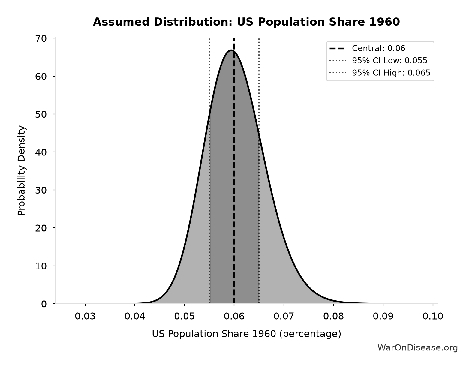
This chart shows the assumed probability distribution for this parameter. The shaded region represents the 95% confidence interval where we expect the true value to fall.
✓ High confidence
Phase 3 Cost per Patient: $41,000
Note📊 Details
Phase 3 cost per patient (median from FDA study)
Source:33
Uncertainty Range
Technical: 95% CI: [$20,000, $120,000] • Distribution: Lognormal
What this means: This estimate is highly uncertain. The true value likely falls between $20,000 and $120,000 (±122%). This represents a very wide range that our Monte Carlo simulations account for when calculating overall uncertainty in the results.
The lognormal distribution means values can’t go negative and have a longer tail toward higher values (common for costs and populations).
Input Distribution
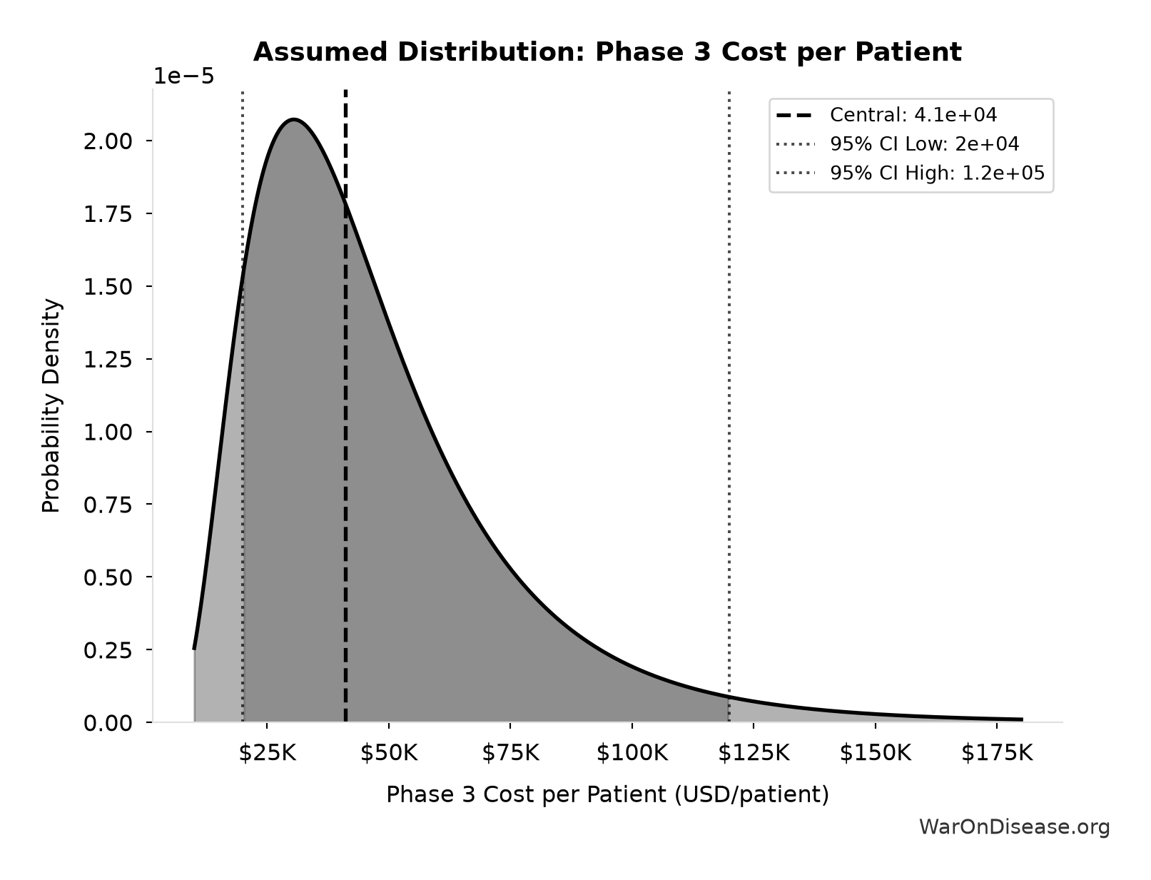
This chart shows the assumed probability distribution for this parameter. The shaded region represents the 95% confidence interval where we expect the true value to fall.
✓ High confidence
Treatment Disability Reduction: 0.25 weight
Note📊 Details
Average disability weight reduction from pharmaceutical treatment. Untreated chronic disease averages 0.35 disability weight, treated disease averages 0.10, difference is 0.25.
Source:44
Uncertainty Range
Technical: 95% CI: [0.15 weight, 0.35 weight] • Distribution: Normal
What this means: There’s significant uncertainty here. The true value likely falls between 0.15 weight and 0.35 weight (±40%). This represents a wide range that our Monte Carlo simulations account for when calculating overall uncertainty in the results.
The normal distribution means values cluster around the center with equal chances of being higher or lower.
Input Distribution
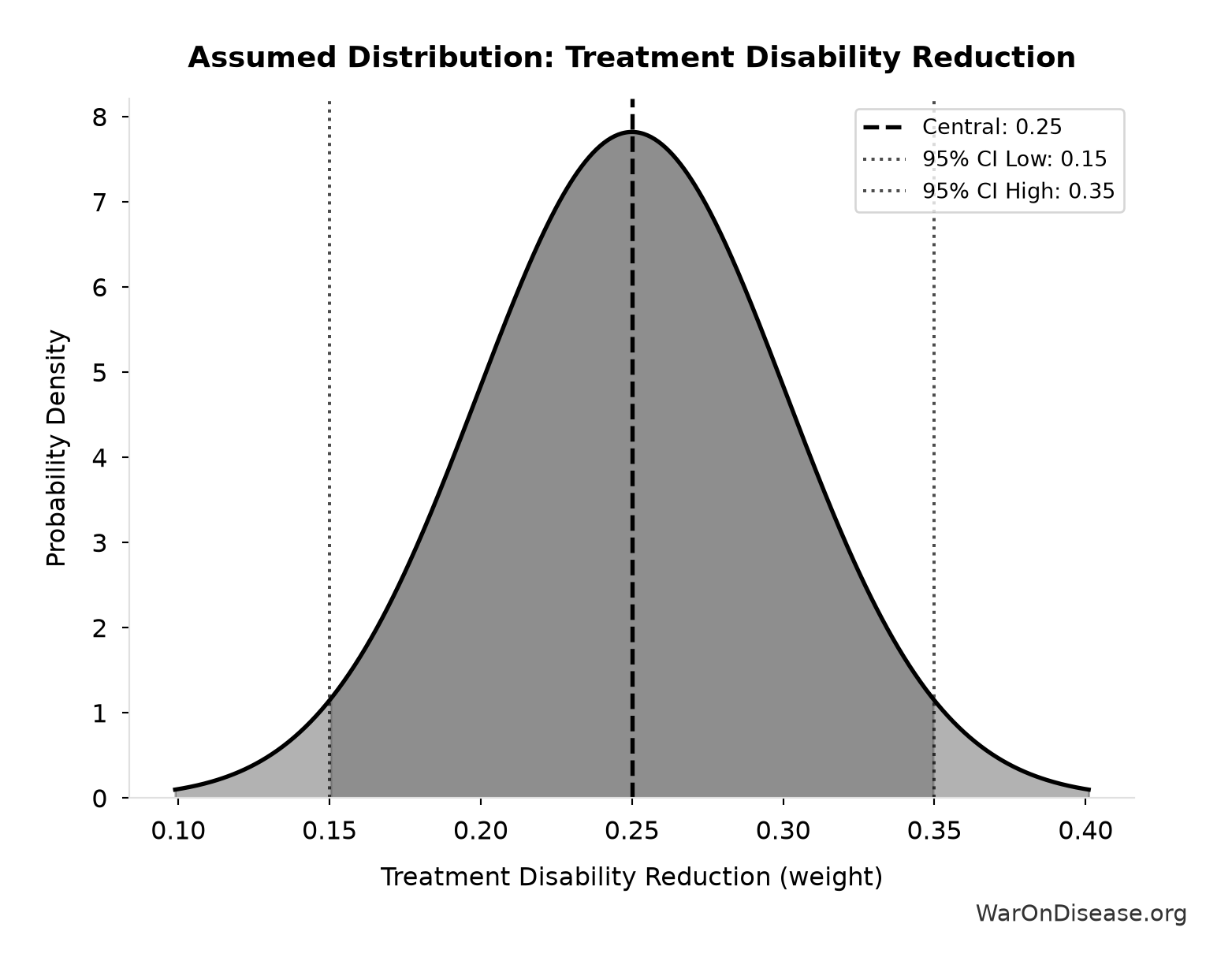
This chart shows the assumed probability distribution for this parameter. The shaded region represents the 95% confidence interval where we expect the true value to fall.
~ Medium confidence • 📊 Peer-reviewed
Value of Statistical Life: $10 million
Note📊 Details
Value of Statistical Life (conservative estimate)
Source:34
Uncertainty Range
Technical: 95% CI: [$5 million, $15 million] • Distribution: Gamma (SE: $3 million)
What this means: There’s significant uncertainty here. The true value likely falls between $5 million and $15 million (±50%). This represents a wide range that our Monte Carlo simulations account for when calculating overall uncertainty in the results.
The gamma distribution means values follow a specific statistical pattern.
Input Distribution
This chart shows the assumed probability distribution for this parameter. The shaded region represents the 95% confidence interval where we expect the true value to fall.
✓ High confidence
Core Definitions
Fundamental parameters and constants used throughout the analysis.
ADAPTABLE Trial Patients Enrolled: 15,076 patients
Note📊 Details
Patients enrolled in ADAPTABLE trial (PCORnet 2016-2019). Enrolled across 40 clinical sites. Precise count from trial completion records.
Core definition
Average Life Extension per Beneficiary: 12 years
Note📊 Details
Average years of life extension per person saved by pharmaceutical interventions. Assumption used to convert life-years saved to approximate lives saved. Based on Lichtenberg’s methodology where life-years are calculated from Years of Life Lost (YLL) reductions.
Uncertainty Range
Technical: 95% CI: [8 years, 18 years] • Distribution: Triangular
What this means: There’s significant uncertainty here. The true value likely falls between 8 years and 18 years (±42%). This represents a wide range that our Monte Carlo simulations account for when calculating overall uncertainty in the results.
The triangular distribution means values cluster around a most-likely point but can range higher or lower.
Input Distribution
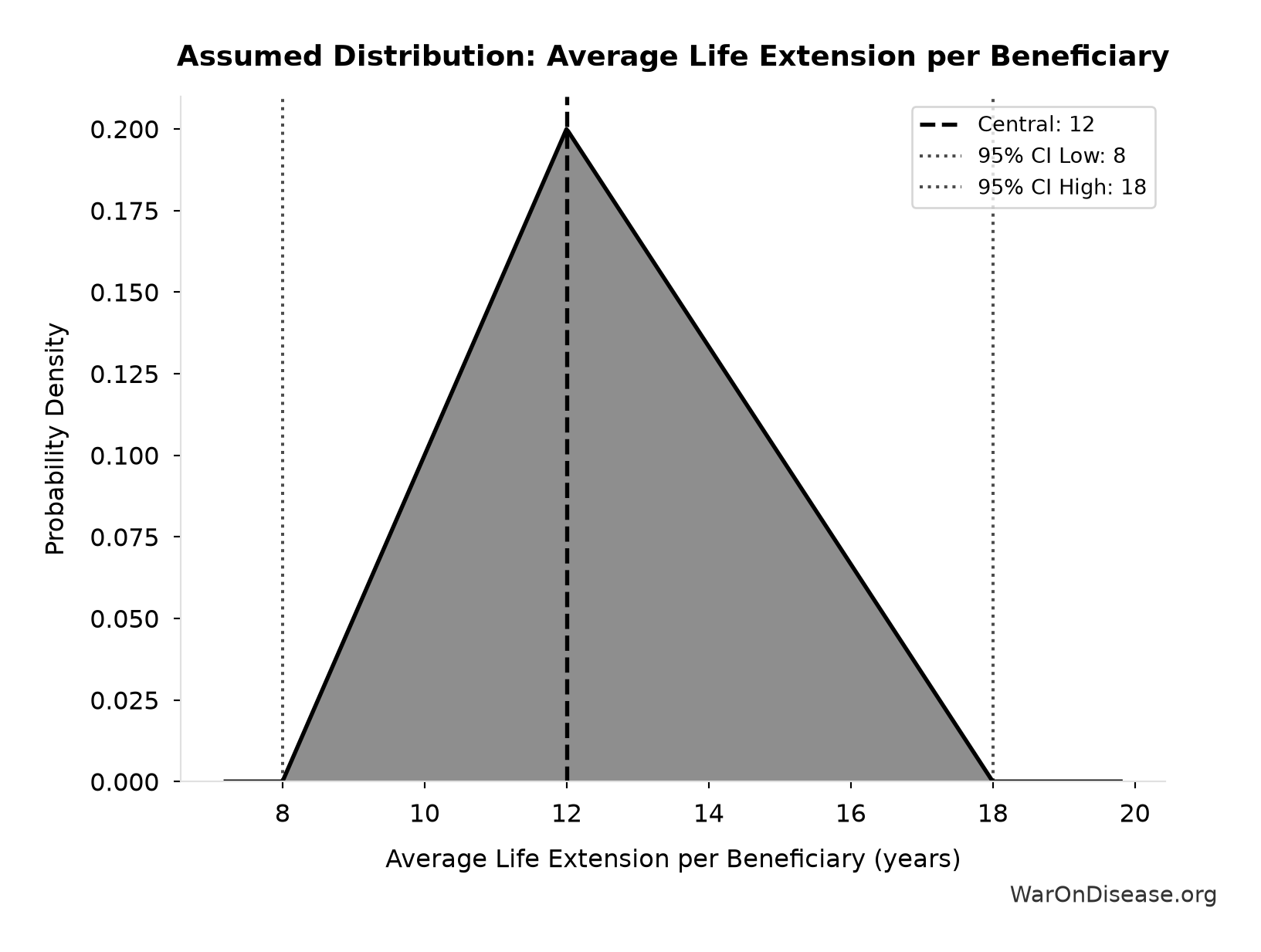
This chart shows the assumed probability distribution for this parameter. The shaded region represents the 95% confidence interval where we expect the true value to fall.
Core definition
Reference Annual Pragmatic Trial Funding: $21.8 billion
Note📊 Details
Reference annual funding level used for direct-funding comparisons. Source-agnostic: funds could come from treaty reallocation, philanthropy, or public appropriation, and are modeled as funding available for pragmatic clinical trials rather than funding owed to any one organization.
Uncertainty Range
Technical: Distribution: Fixed
Core definition
Pragmatic Trial Platform Core Framework Annual OPEX: $18.9 million
Note📊 Details
Pragmatic trial platform core framework annual opex (midpoint of $11-26.5M)
Uncertainty Range
Technical: 95% CI: [$11 million, $26.5 million] • Distribution: Lognormal
What this means: There’s significant uncertainty here. The true value likely falls between $11 million and $26.5 million (±41%). This represents a wide range that our Monte Carlo simulations account for when calculating overall uncertainty in the results.
The lognormal distribution means values can’t go negative and have a longer tail toward higher values (common for costs and populations).
Input Distribution
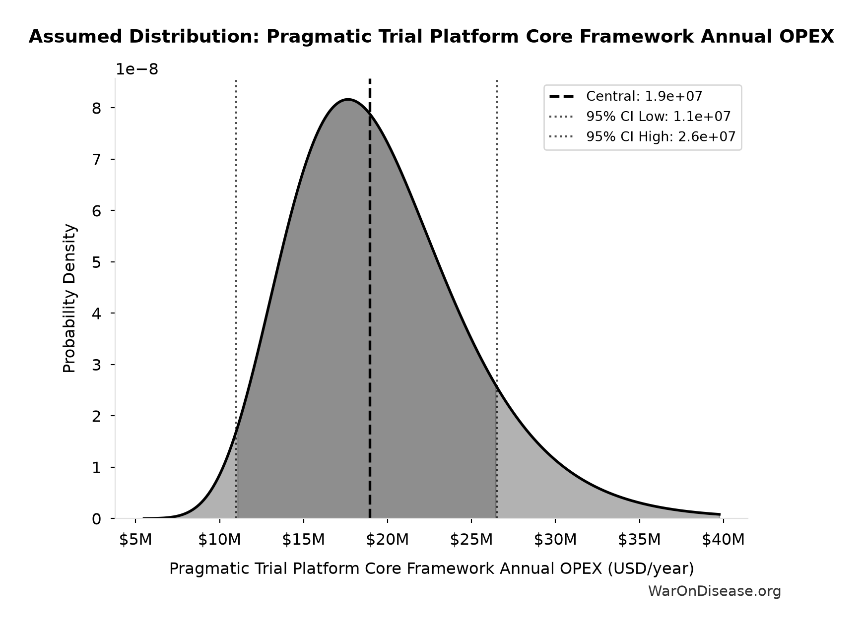
This chart shows the assumed probability distribution for this parameter. The shaded region represents the 95% confidence interval where we expect the true value to fall.
Core definition
Pragmatic Trial Platform Core Framework Build Cost: $40 million
Note📊 Details
Pragmatic trial platform core framework build cost
Uncertainty Range
Technical: 95% CI: [$25 million, $65 million] • Distribution: Lognormal
What this means: There’s significant uncertainty here. The true value likely falls between $25 million and $65 million (±50%). This represents a wide range that our Monte Carlo simulations account for when calculating overall uncertainty in the results.
The lognormal distribution means values can’t go negative and have a longer tail toward higher values (common for costs and populations).
Input Distribution
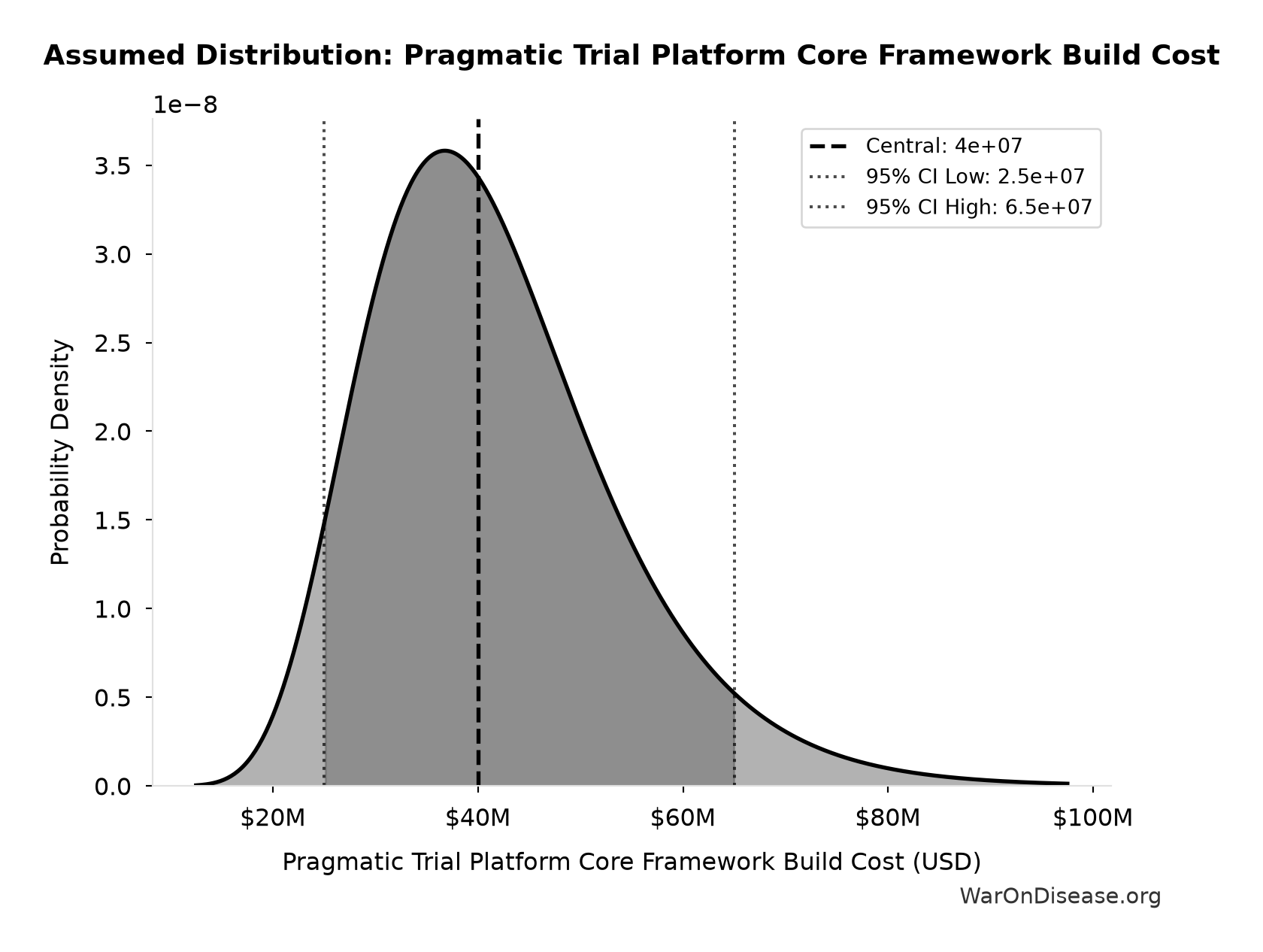
This chart shows the assumed probability distribution for this parameter. The shaded region represents the 95% confidence interval where we expect the true value to fall.
Core definition
Stage 1 Observational Analysis Cost per Patient: $0.1
Note📊 Details
Order-of-magnitude estimate for Stage 1 observational signal detection (PIS calculation). Validated by FDA Sentinel benchmark (~$1/patient/year for similar drug safety analysis at 100M+ scale). True cost varies with scale and complexity; exact value less important than order-of-magnitude difference vs pragmatic trials (~$500-929/patient) and traditional Phase 3 (~$41,000/patient).
Uncertainty Range
Technical: 95% CI: [$0.03, $1] • Distribution: Lognormal
What this means: This estimate is highly uncertain. The true value likely falls between $0.03 and $1 (±485%). This represents a very wide range that our Monte Carlo simulations account for when calculating overall uncertainty in the results.
The lognormal distribution means values can’t go negative and have a longer tail toward higher values (common for costs and populations).
Input Distribution
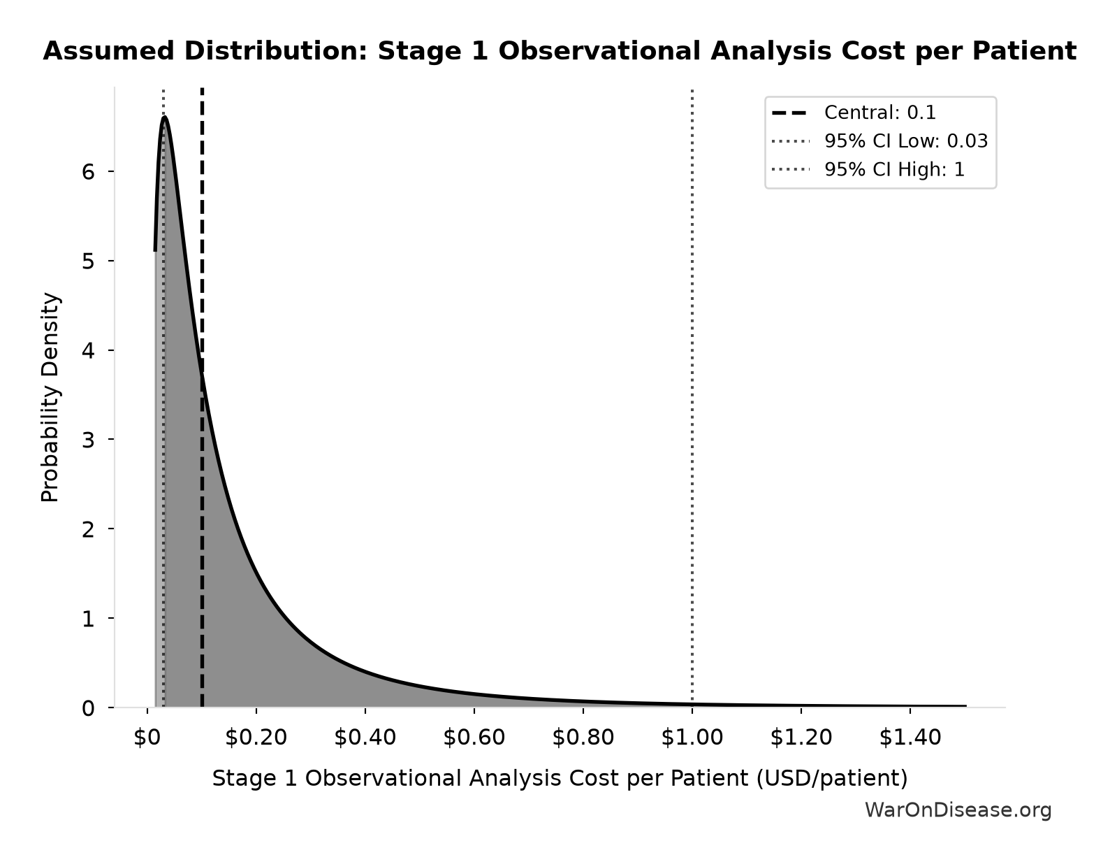
This chart shows the assumed probability distribution for this parameter. The shaded region represents the 95% confidence interval where we expect the true value to fall.
Core definition
Pragmatic Trial Platform Community Support Costs: $2 million
Note📊 Details
Pragmatic trial platform community support costs
Uncertainty Range
Technical: 95% CI: [$1 million, $3 million] • Distribution: Lognormal
What this means: There’s significant uncertainty here. The true value likely falls between $1 million and $3 million (±50%). This represents a wide range that our Monte Carlo simulations account for when calculating overall uncertainty in the results.
The lognormal distribution means values can’t go negative and have a longer tail toward higher values (common for costs and populations).
Input Distribution
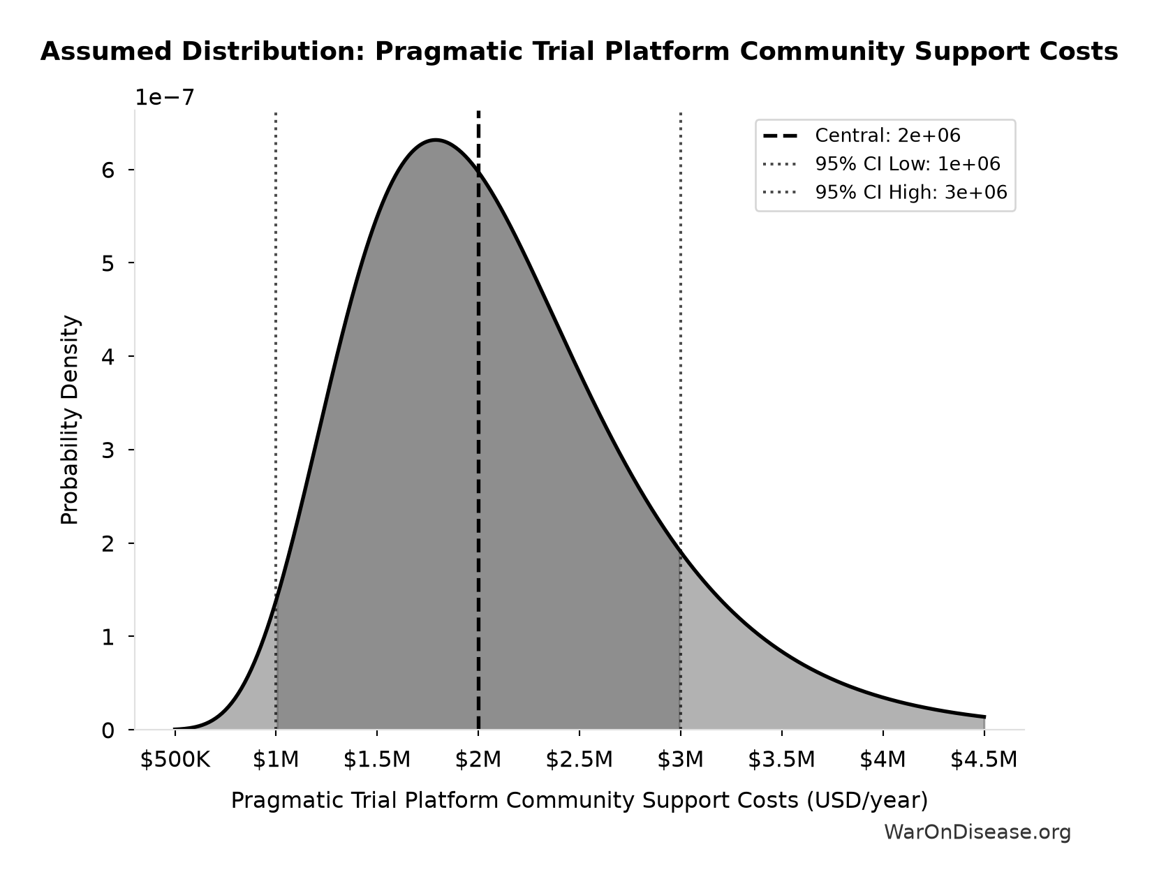
This chart shows the assumed probability distribution for this parameter. The shaded region represents the 95% confidence interval where we expect the true value to fall.
Core definition
Pragmatic Trial Platform Infrastructure Costs: $8 million
Note📊 Details
Pragmatic trial platform infrastructure costs (cloud, security)
Uncertainty Range
Technical: 95% CI: [$5 million, $12 million] • Distribution: Lognormal
What this means: There’s significant uncertainty here. The true value likely falls between $5 million and $12 million (±44%). This represents a wide range that our Monte Carlo simulations account for when calculating overall uncertainty in the results.
The lognormal distribution means values can’t go negative and have a longer tail toward higher values (common for costs and populations).
Input Distribution
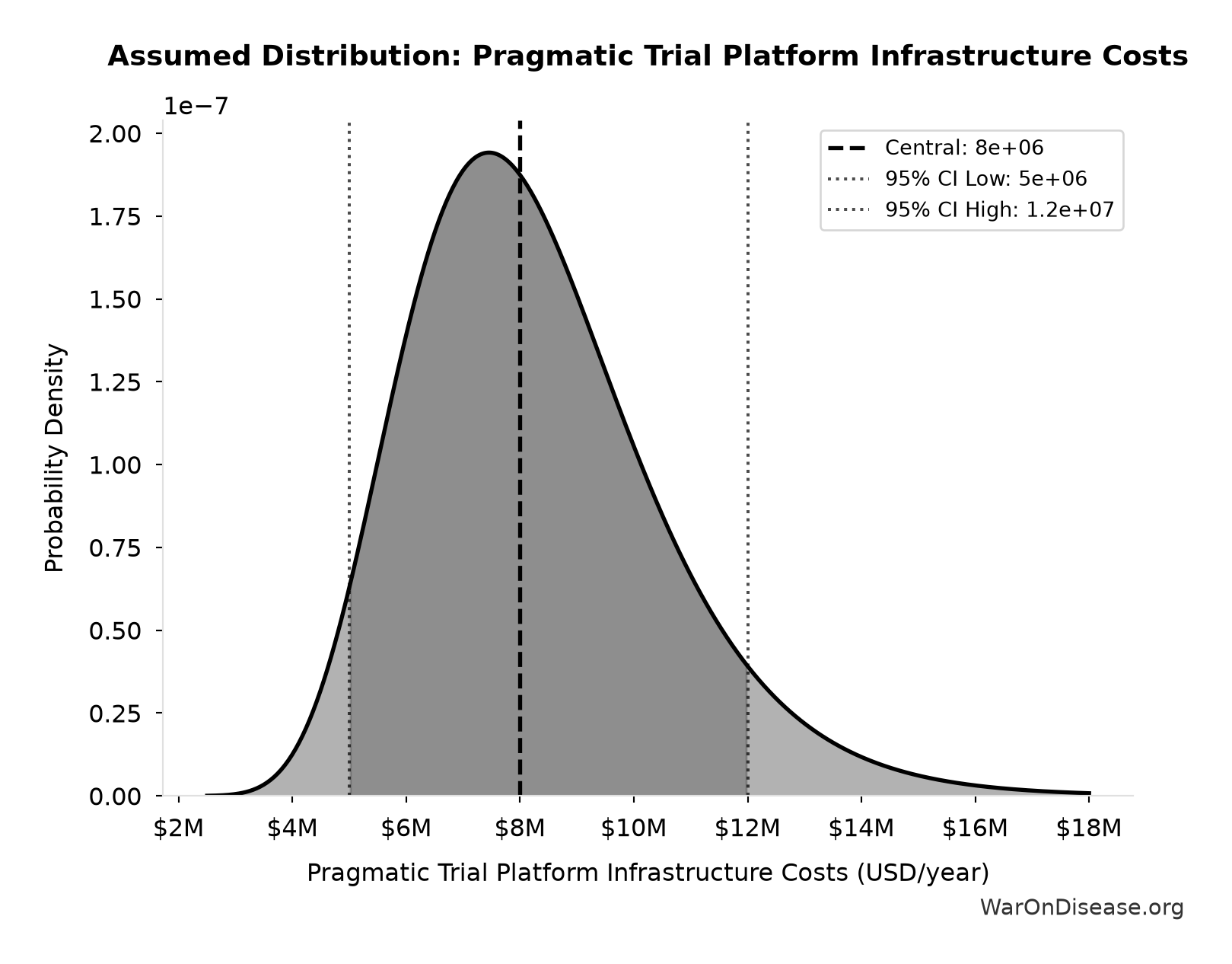
This chart shows the assumed probability distribution for this parameter. The shaded region represents the 95% confidence interval where we expect the true value to fall.
Core definition
Pragmatic Trial Platform Maintenance Costs: $15 million
Note📊 Details
Pragmatic trial platform maintenance costs
Uncertainty Range
Technical: 95% CI: [$10 million, $22 million] • Distribution: Lognormal
What this means: There’s significant uncertainty here. The true value likely falls between $10 million and $22 million (±40%). This represents a wide range that our Monte Carlo simulations account for when calculating overall uncertainty in the results.
The lognormal distribution means values can’t go negative and have a longer tail toward higher values (common for costs and populations).
Input Distribution
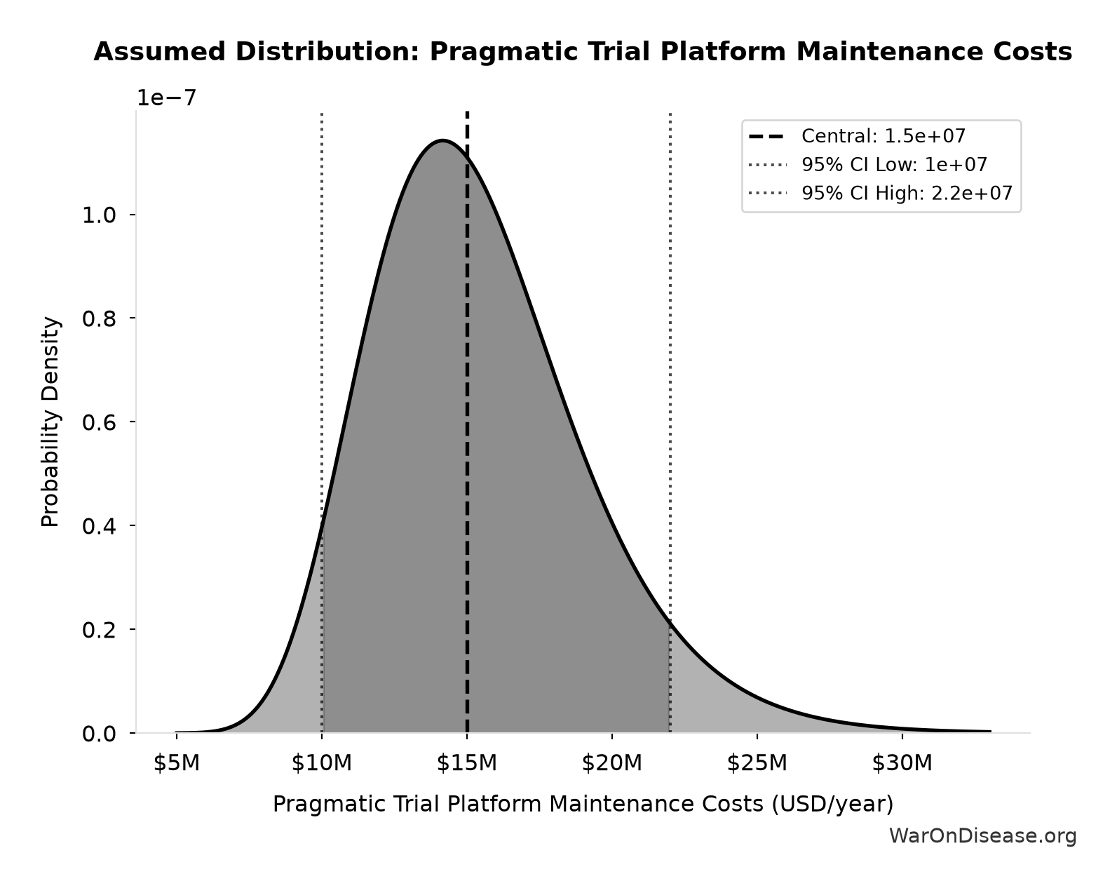
This chart shows the assumed probability distribution for this parameter. The shaded region represents the 95% confidence interval where we expect the true value to fall.
Core definition
Pragmatic Trial Platform Regulatory Coordination Costs: $5 million
Note📊 Details
Pragmatic trial platform regulatory coordination costs
Uncertainty Range
Technical: 95% CI: [$3 million, $8 million] • Distribution: Lognormal
What this means: There’s significant uncertainty here. The true value likely falls between $3 million and $8 million (±50%). This represents a wide range that our Monte Carlo simulations account for when calculating overall uncertainty in the results.
The lognormal distribution means values can’t go negative and have a longer tail toward higher values (common for costs and populations).
Input Distribution
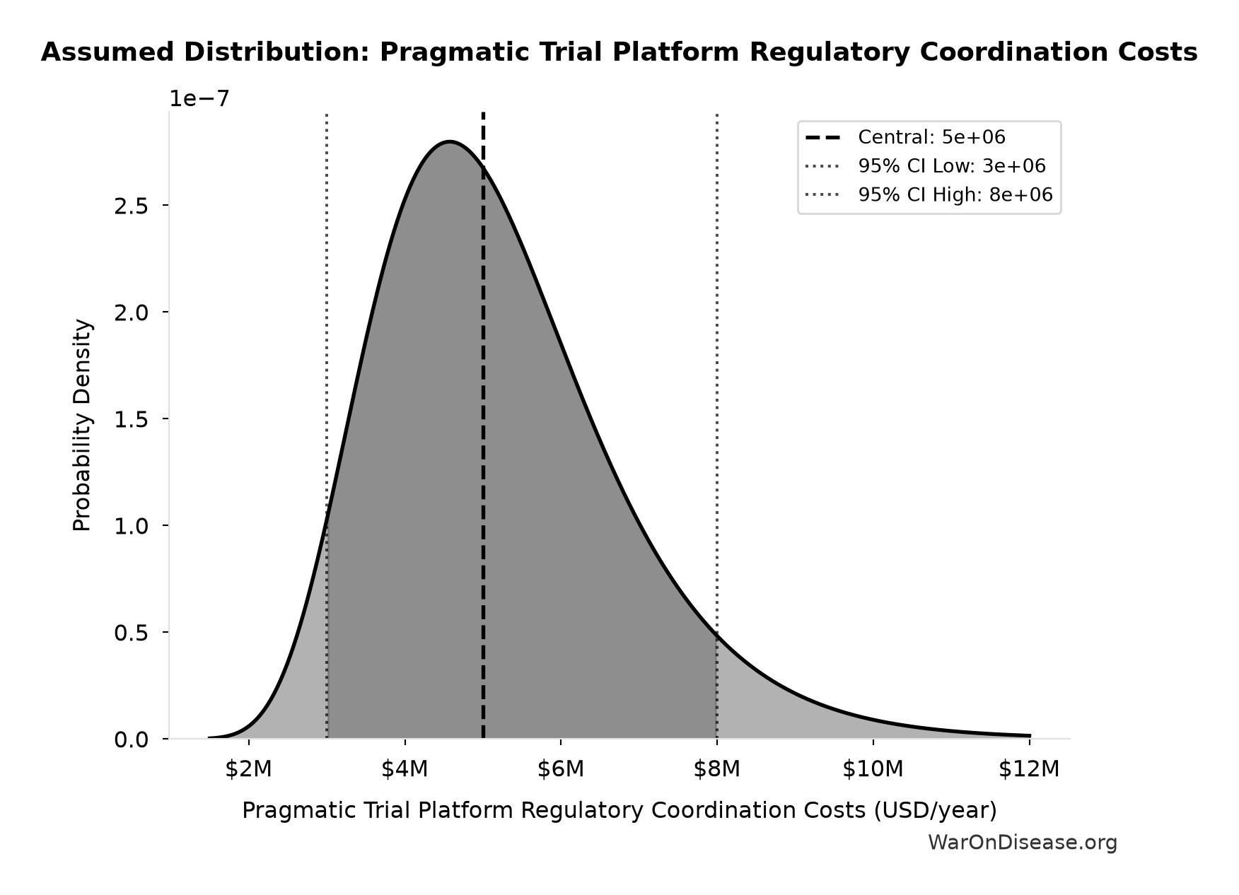
This chart shows the assumed probability distribution for this parameter. The shaded region represents the 95% confidence interval where we expect the true value to fall.
Core definition
Pragmatic Trial Platform Staff Costs: $10 million
Note📊 Details
Pragmatic trial platform staff costs (minimal, AI-assisted)
Uncertainty Range
Technical: 95% CI: [$7 million, $15 million] • Distribution: Lognormal
What this means: There’s significant uncertainty here. The true value likely falls between $7 million and $15 million (±40%). This represents a wide range that our Monte Carlo simulations account for when calculating overall uncertainty in the results.
The lognormal distribution means values can’t go negative and have a longer tail toward higher values (common for costs and populations).
Input Distribution
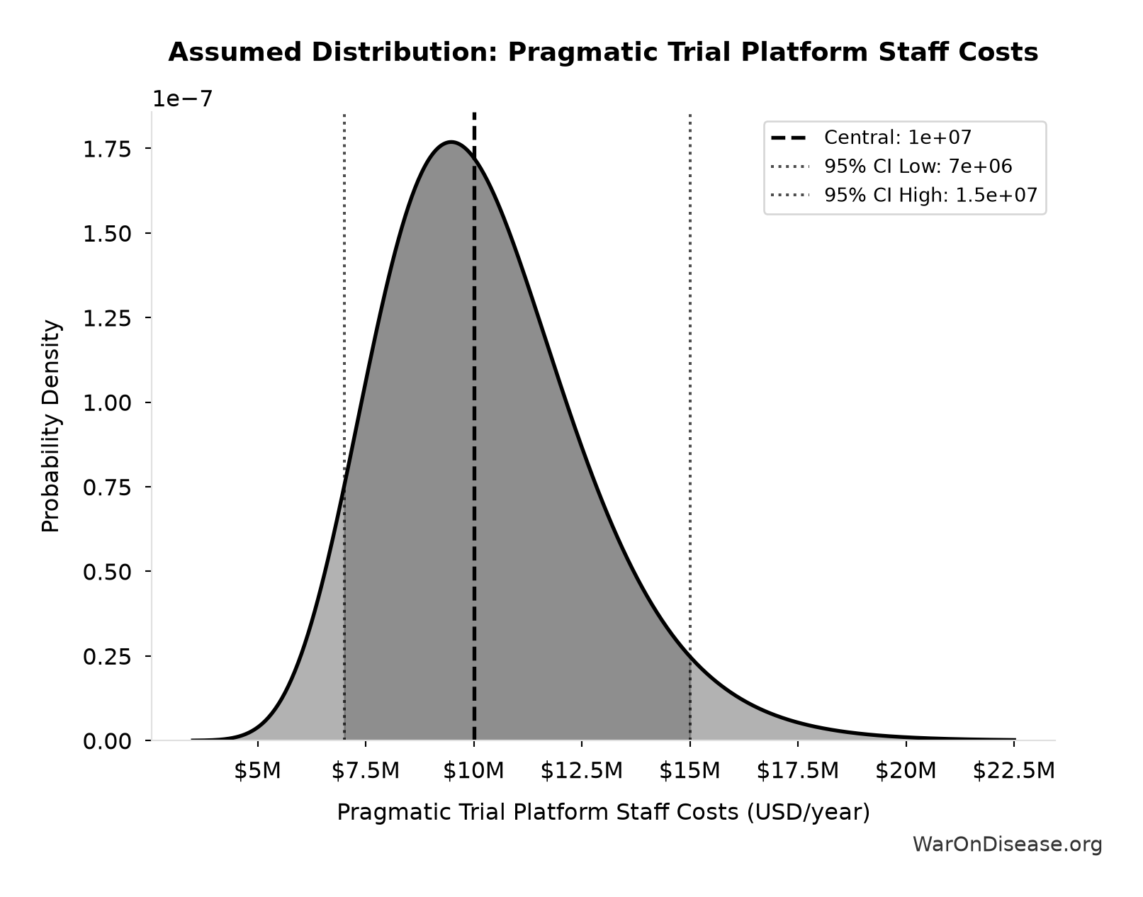
This chart shows the assumed probability distribution for this parameter. The shaded region represents the 95% confidence interval where we expect the true value to fall.
Core definition
Pragmatic Trial Platform One-Time Build Cost (Maximum): $46 million
Note📊 Details
Pragmatic trial platform one-time build cost (high estimate)
Core definition
DIH Broader Initiatives Annual OPEX: $21.1 million
Note📊 Details
DIH broader initiatives annual opex (medium case)
Uncertainty Range
Technical: 95% CI: [$14 million, $32 million] • Distribution: Lognormal
What this means: There’s significant uncertainty here. The true value likely falls between $14 million and $32 million (±43%). This represents a wide range that our Monte Carlo simulations account for when calculating overall uncertainty in the results.
The lognormal distribution means values can’t go negative and have a longer tail toward higher values (common for costs and populations).
Input Distribution
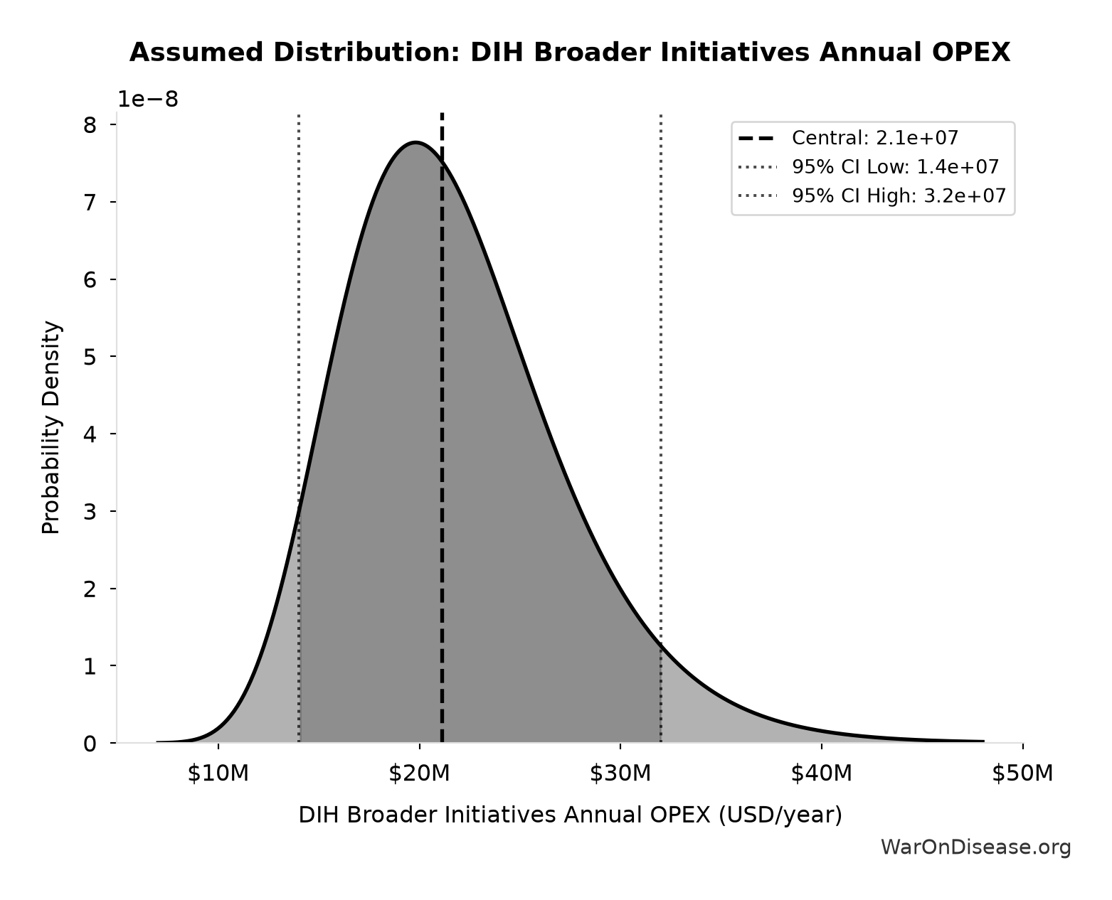
This chart shows the assumed probability distribution for this parameter. The shaded region represents the 95% confidence interval where we expect the true value to fall.
Core definition
DIH Broader Initiatives Upfront Cost: $230 million
Note📊 Details
DIH broader initiatives upfront cost (medium case)
Uncertainty Range
Technical: 95% CI: [$150 million, $350 million] • Distribution: Lognormal
What this means: There’s significant uncertainty here. The true value likely falls between $150 million and $350 million (±44%). This represents a wide range that our Monte Carlo simulations account for when calculating overall uncertainty in the results.
The lognormal distribution means values can’t go negative and have a longer tail toward higher values (common for costs and populations).
Input Distribution
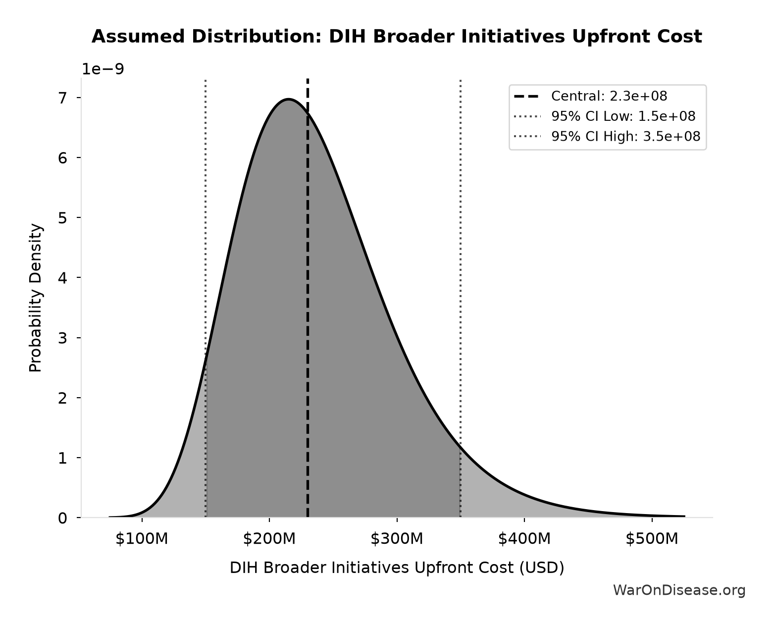
This chart shows the assumed probability distribution for this parameter. The shaded region represents the 95% confidence interval where we expect the true value to fall.
Core definition
Eventually Avoidable DALY Percentage: 92.6%
Note📊 Details
Percentage of DALYs that are eventually avoidable with sufficient biomedical research. Uses same methodology as EVENTUALLY_AVOIDABLE_DEATH_PCT. Most non-fatal chronic conditions (arthritis, depression, chronic pain) are also addressable through research, so the percentage is similar to deaths.
Uncertainty Range
Technical: 95% CI: [50%, 98%] • Distribution: Beta
What this means: There’s significant uncertainty here. The true value likely falls between 50% and 98% (±26%). This represents a wide range that our Monte Carlo simulations account for when calculating overall uncertainty in the results.
The beta distribution means values are bounded and can skew toward one end.
Input Distribution
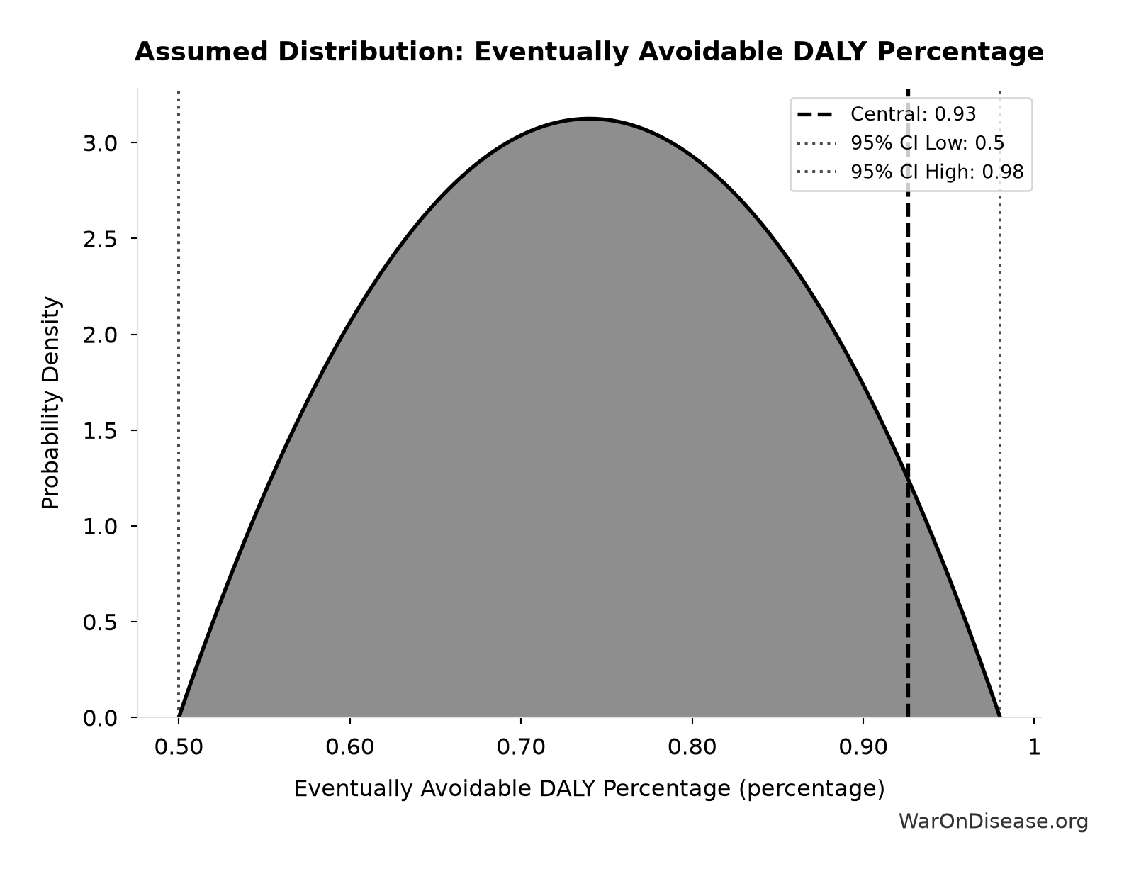
This chart shows the assumed probability distribution for this parameter. The shaded region represents the 95% confidence interval where we expect the true value to fall.
Core definition
Eventually Avoidable Death Percentage: 92.6%
Note📊 Details
Percentage of deaths that are eventually avoidable with sufficient biomedical research and technological advancement. Central estimate ~92% based on ~7.9% fundamentally unavoidable (primarily accidents). Wide uncertainty reflects debate over: (1) aging as addressable vs. fundamental, (2) asymptotic difficulty of last diseases, (3) multifactorial disease complexity.
Uncertainty Range
Technical: 95% CI: [50%, 98%] • Distribution: Beta
What this means: There’s significant uncertainty here. The true value likely falls between 50% and 98% (±26%). This represents a wide range that our Monte Carlo simulations account for when calculating overall uncertainty in the results.
The beta distribution means values are bounded and can skew toward one end.
Input Distribution
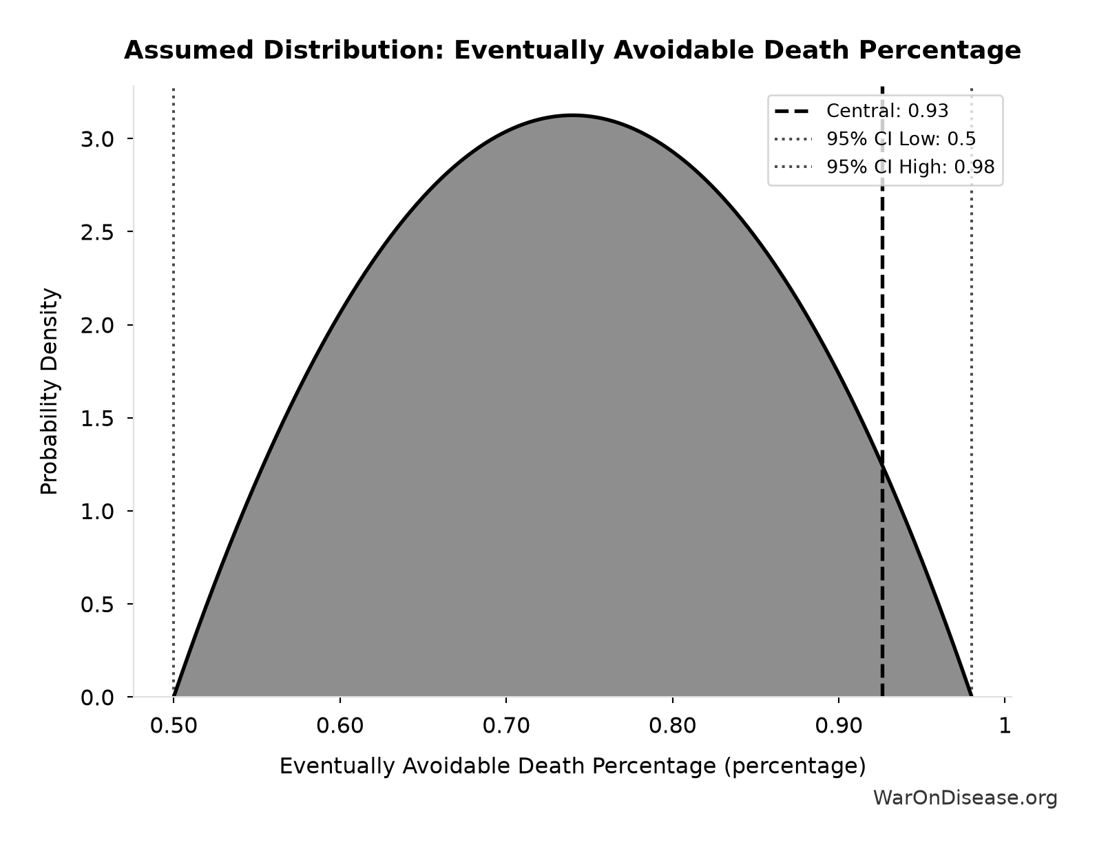
This chart shows the assumed probability distribution for this parameter. The shaded region represents the 95% confidence interval where we expect the true value to fall.
Core definition
Standard Discount Rate for NPV Analysis: 3%
Note📊 Details
Standard discount rate for NPV analysis (3% annual, social discount rate)
Uncertainty Range
Technical: Distribution: Fixed
Core definition
Standard Time Horizon for NPV Analysis: 10 years
Note📊 Details
Standard time horizon for NPV analysis
Uncertainty Range
Technical: Distribution: Fixed
Core definition
Pharma Phase 2/3 Cost Barrier Per Drug: $1.56 billion
Note📊 Details
Average Phase 2/3 efficacy testing cost per drug that pharma must fund (~60% of total drug development cost)
Uncertainty Range
Technical: Distribution: Normal (SE: $200 million)
Input Distribution
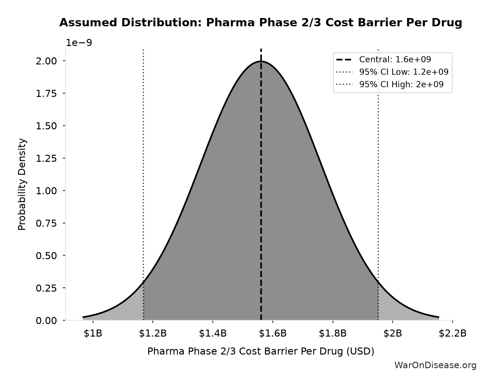
This chart shows the assumed probability distribution for this parameter. The shaded region represents the 95% confidence interval where we expect the true value to fall.
Core definition
QALYs per COVID Death Averted: 5 QALYs/death
Note📊 Details
Average QALYs gained per COVID death averted. Conservative estimate reflecting older age distribution of COVID mortality. See confidence_interval for range.
Uncertainty Range
Technical: 95% CI: [3 QALYs/death, 10 QALYs/death] • Distribution: Lognormal
What this means: This estimate is highly uncertain. The true value likely falls between 3 QALYs/death and 10 QALYs/death (±70%). This represents a very wide range that our Monte Carlo simulations account for when calculating overall uncertainty in the results.
The lognormal distribution means values can’t go negative and have a longer tail toward higher values (common for costs and populations).
Input Distribution
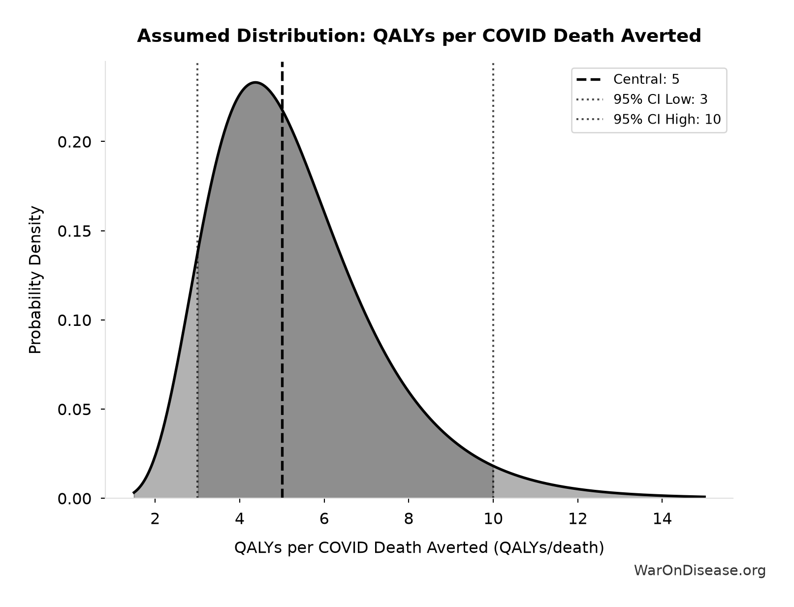
This chart shows the assumed probability distribution for this parameter. The shaded region represents the 95% confidence interval where we expect the true value to fall.
Core definition
Safe Compounds Available for Testing: 9,500 compounds
Note📊 Details
Total safe compounds available for repurposing (FDA-approved + GRAS substances, midpoint of 7,000-12,000 range)
Uncertainty Range
Technical: 95% CI: [7,000 compounds, 12,000 compounds] • Distribution: Uniform
What this means: There’s significant uncertainty here. The true value likely falls between 7,000 compounds and 12,000 compounds (±26%). This represents a wide range that our Monte Carlo simulations account for when calculating overall uncertainty in the results.
The uniform distribution means any value in the range is equally likely.
Input Distribution
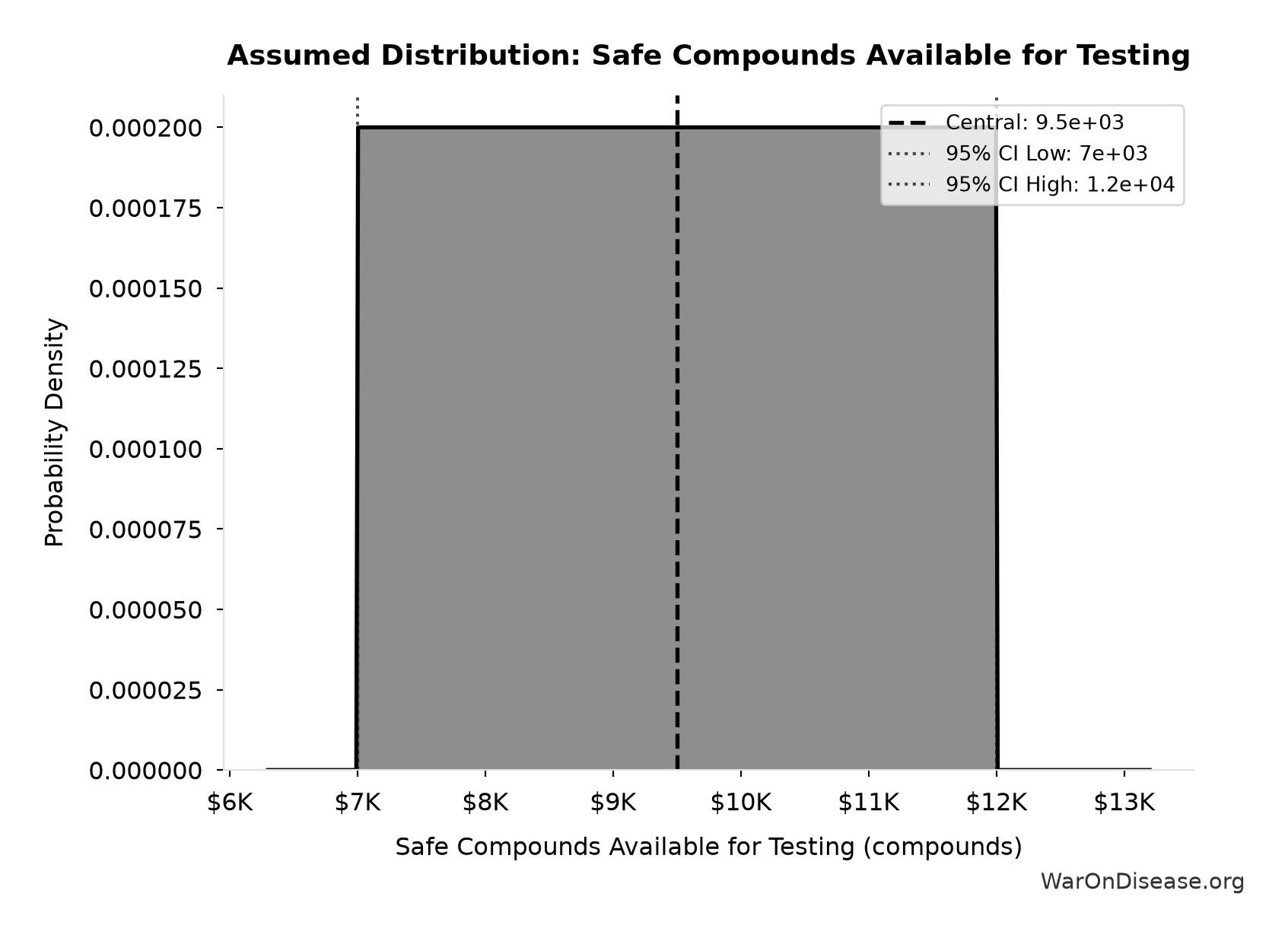
This chart shows the assumed probability distribution for this parameter. The shaded region represents the 95% confidence interval where we expect the true value to fall.
Core definition
Universal Right to Try with Evidence Implementation Cost: $65 million
Note📊 Details
Total implementation cost of adopting Universal Right to Try with Evidence in all 50 states: a central $15 million campaign estimate covering legislation or amendment in all 50 states plus $50 million for the shared registry’s first ten years. The model bill requires participating centers to fund continued registry operation after year ten. This launch-cost numerator excludes patient or payer spending on treatment delivery, trial-site services, and permitted study costs. The wide interval represents campaign and infrastructure cost uncertainty without separate scenario parameters.
Uncertainty Range
Technical: 95% CI: [$25 million, $200 million] • Distribution: Lognormal
What this means: This estimate is highly uncertain. The true value likely falls between $25 million and $200 million (±135%). This represents a very wide range that our Monte Carlo simulations account for when calculating overall uncertainty in the results.
The lognormal distribution means values can’t go negative and have a longer tail toward higher values (common for costs and populations).
Input Distribution
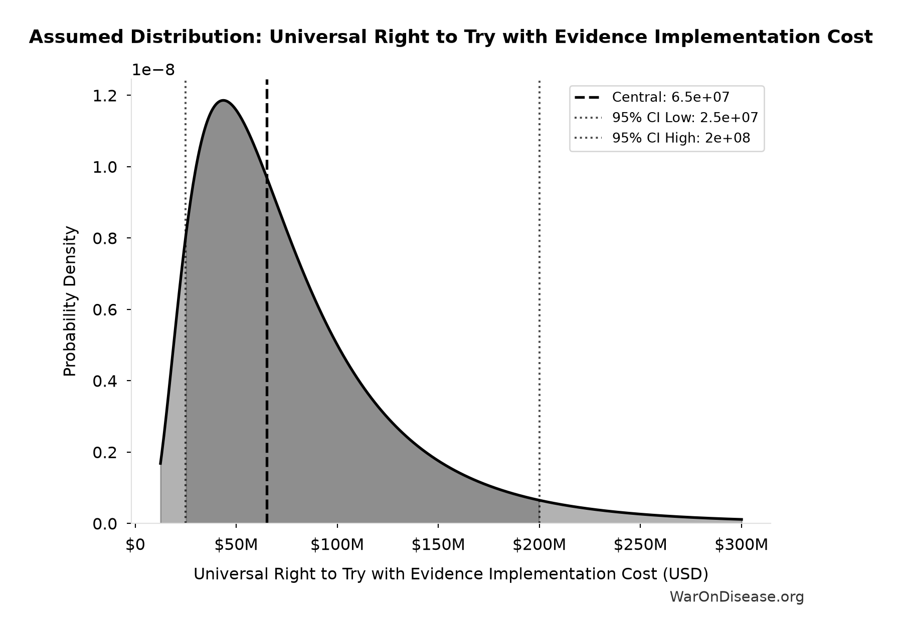
This chart shows the assumed probability distribution for this parameter. The shaded region represents the 95% confidence interval where we expect the true value to fall.
Core definition
Universal Right to Try with Evidence Treatment Discovery Multiplier: 5.48x
Note📊 Details
Conditional multiplier on the worldwide first-treatment discovery rate after all 50 states adopt and a mature pooled pragmatic-trial system operates under applicable federal authorization. The 5.48x central calibration reproduces the prior model’s 82.2 versus 15 first treatments per year; it is an assumption, not an observed effect estimate. This single input incorporates patient or payer funding of treatment delivery, trial-site services, and permitted study costs, newly viable post-Phase-1 treatment-condition pairs, evaluable protocol quality, candidate supply, and scientific success. Its range describes productivity of an operating system, not the separate probability that advocacy achieves full adoption and implementation.
Uncertainty Range
Technical: 95% CI: [1.1x, 15x] • Distribution: Lognormal
What this means: This estimate is highly uncertain. The true value likely falls between 1.1x and 15x (±127%). This represents a very wide range that our Monte Carlo simulations account for when calculating overall uncertainty in the results.
The lognormal distribution means values can’t go negative and have a longer tail toward higher values (common for costs and populations).
Input Distribution
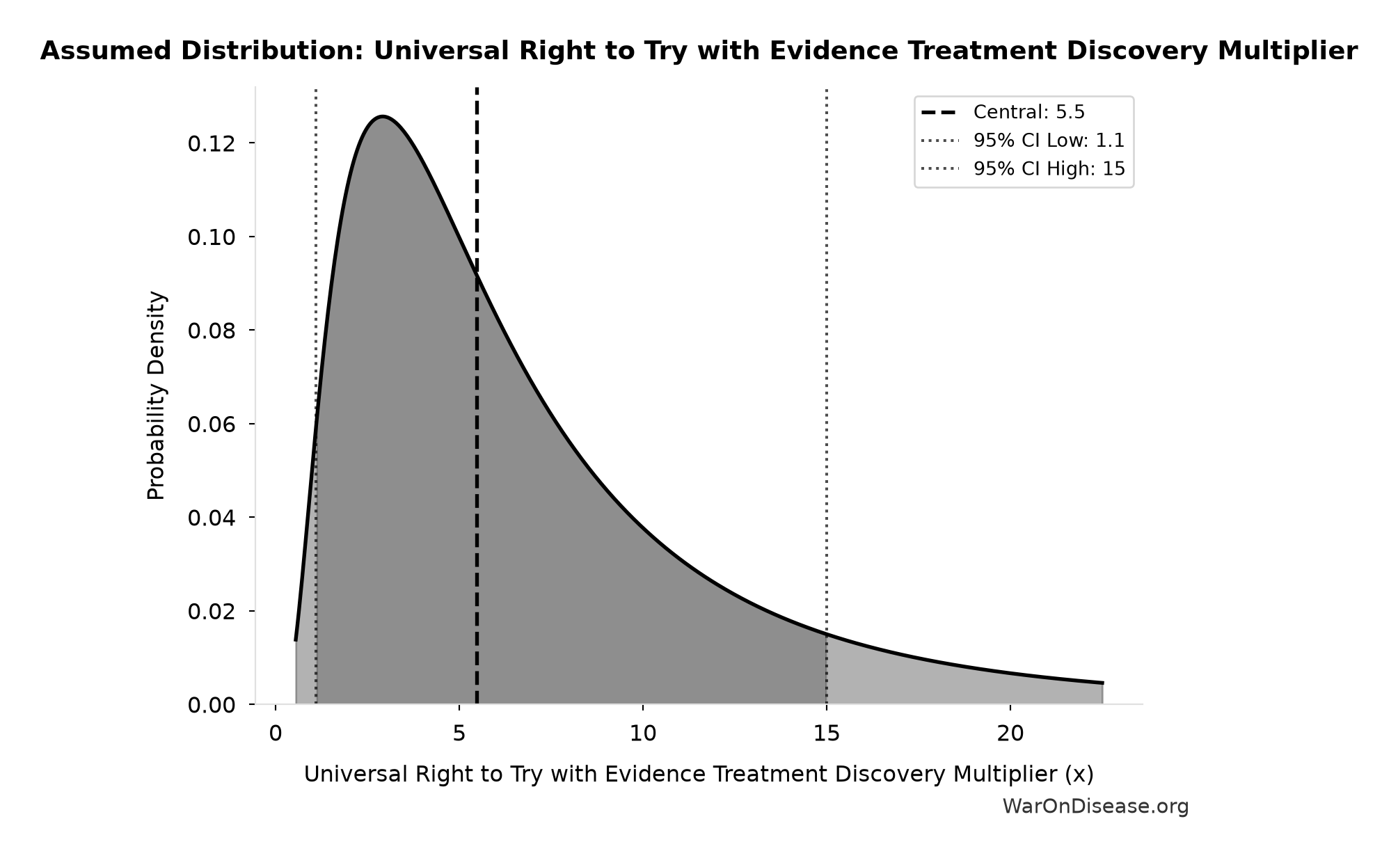
This chart shows the assumed probability distribution for this parameter. The shaded region represents the 95% confidence interval where we expect the true value to fall.
Core definition
Tested Drug-Disease Relationships: 32,500 relationships
Note📊 Details
Estimated drug-disease relationships actually tested (approved uses + repurposed + failed trials, midpoint of 15,000-50,000 range)
Uncertainty Range
Technical: 95% CI: [15,000 relationships, 50,000 relationships] • Distribution: Lognormal
What this means: This estimate is highly uncertain. The true value likely falls between 15,000 relationships and 50,000 relationships (±54%). This represents a very wide range that our Monte Carlo simulations account for when calculating overall uncertainty in the results.
The lognormal distribution means values can’t go negative and have a longer tail toward higher values (common for costs and populations).
Input Distribution
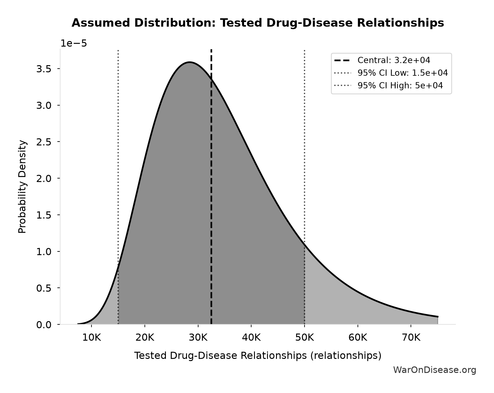
This chart shows the assumed probability distribution for this parameter. The shaded region represents the 95% confidence interval where we expect the true value to fall.
Core definition
Trial-Relevant Diseases: 1,000 diseases
Note📊 Details
Consolidated count of trial-relevant diseases worth targeting (after grouping ICD-10 codes)
Uncertainty Range
Technical: 95% CI: [800 diseases, 1,200 diseases] • Distribution: Uniform
What this means: This estimate has moderate uncertainty. The true value likely falls between 800 diseases and 1,200 diseases (±20%). This represents a reasonable range that our Monte Carlo simulations account for when calculating overall uncertainty in the results.
The uniform distribution means any value in the range is equally likely.
Input Distribution
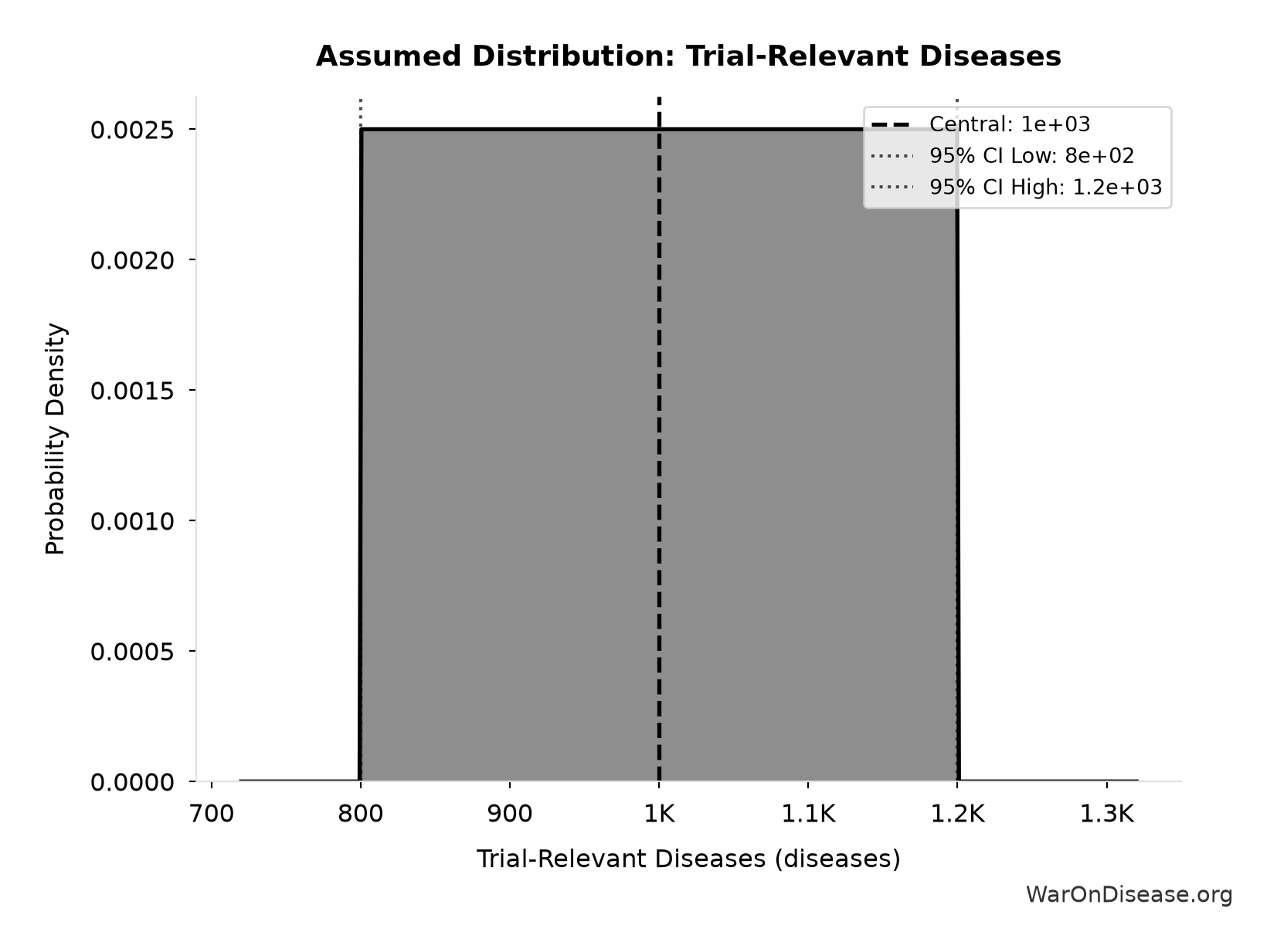
This chart shows the assumed probability distribution for this parameter. The shaded region represents the 95% confidence interval where we expect the true value to fall.
Core definition
References
1.
NIH Common Fund. NIH pragmatic trials: Minimal funding despite 30x cost advantage. NIH Common Fund: HCS Research Collaboratory https://commonfund.nih.gov/hcscollaboratory (2025)
The NIH Pragmatic Trials Collaboratory funds trials at $500K for planning phase, $1M/year for implementation-a tiny fraction of NIH’s budget. The ADAPTABLE trial cost $14 million for 15,076 patients (= $929/patient) versus $420 million for a similar traditional RCT (30x cheaper), yet pragmatic trials remain severely underfunded. PCORnet infrastructure enables real-world trials embedded in healthcare systems, but receives minimal support compared to basic research funding. Additional sources: https://commonfund.nih.gov/hcscollaboratory | https://pcornet.org/wp-content/uploads/2025/08/ADAPTABLE_Lay_Summary_21JUL2025.pdf | https://www.ncbi.nlm.nih.gov/pmc/articles/PMC5604499/
.2.
NIH. Antidepressant clinical trial exclusion rates. Zimmerman et al. https://pubmed.ncbi.nlm.nih.gov/26276679/ (2015)
Mean exclusion rate: 86.1% across 158 antidepressant efficacy trials (range: 44.4% to 99.8%) More than 82% of real-world depression patients would be ineligible for antidepressant registration trials Exclusion rates increased over time: 91.4% (2010-2014) vs. 83.8% (1995-2009) Most common exclusions: comorbid psychiatric disorders, age restrictions, insufficient depression severity, medical conditions Emergency psychiatry patients: only 3.3% eligible (96.7% excluded) when applying 9 common exclusion criteria Only a minority of depressed patients seen in clinical practice are likely to be eligible for most AETs Note: Generalizability of antidepressant trials has decreased over time, with increasingly stringent exclusion criteria eliminating patients who would actually use the drugs in clinical practice Additional sources: https://pubmed.ncbi.nlm.nih.gov/26276679/ | https://pubmed.ncbi.nlm.nih.gov/26164052/ | https://www.wolterskluwer.com/en/news/antidepressant-trials-exclude-most-real-world-patients-with-depression
.3.
GiveWell. GiveWell cost per life saved for top charities (2024). GiveWell: Top Charities https://www.givewell.org/charities/top-charities
General range: $3,000-$5,500 per life saved (GiveWell top charities) Helen Keller International (Vitamin A): $3,500 average (2022-2024); varies $1,000-$8,500 by country Against Malaria Foundation: $5,500 per life saved New Incentives (vaccination incentives): $4,500 per life saved Malaria Consortium (seasonal malaria chemoprevention): $3,500 per life saved VAS program details: $2 to provide vitamin A supplements to child for one year Note: Figures accurate for 2024. Helen Keller VAS program has wide country variation ($1K-$8.5K) but $3,500 is accurate average. Among most cost-effective interventions globally Additional sources: https://www.givewell.org/charities/top-charities | https://www.givewell.org/charities/helen-keller-international | https://ourworldindata.org/cost-effectiveness
.4.
World Health Organization. WHO global health estimates 2024. World Health Organization https://www.who.int/data/gho/data/themes/mortality-and-global-health-estimates (2024)
Comprehensive mortality and morbidity data by cause, age, sex, country, and year Global mortality: 55-60 million deaths annually Lives saved by modern medicine (vaccines, cardiovascular drugs, oncology): 12M annually (conservative aggregate) Leading causes of death: Cardiovascular disease (17.9M), Cancer (10.3M), Respiratory disease (4.0M) Note: Baseline data for regulatory mortality analysis. Conservative estimate of pharmaceutical impact based on WHO immunization data (4.5M/year from vaccines) + cardiovascular interventions (3.3M/year) + oncology (1.5M/year) + other therapies. Additional sources: https://www.who.int/data/gho/data/themes/mortality-and-global-health-estimates
.5.
U.S. Bureau of Labor Statistics. CPI inflation calculator. (2024)
CPI-U (1980): 82.4 CPI-U (2024): 313.5 Inflation multiplier (1980-2024): 3.80× Cumulative inflation: 280.48% Average annual inflation rate: 3.08% Note: Official U.S. government inflation data using Consumer Price Index for All Urban Consumers (CPI-U). Additional sources: https://www.bls.gov/data/inflation_calculator.htm
.6.
ACS CAN. Clinical trial patient participation rate. ACS CAN: Barriers to Clinical Trial Enrollment https://www.fightcancer.org/policy-resources/barriers-patient-enrollment-therapeutic-clinical-trials-cancer
Only 3-5% of adult cancer patients in US receive treatment within clinical trials About 5% of American adults have ever participated in any clinical trial Oncology: 2-3% of all oncology patients participate Contrast: 50-60% enrollment for pediatric cancer trials (<15 years old) Note: 20% of cancer trials fail due to insufficient enrollment; 11% of research sites enroll zero patients Additional sources: https://www.fightcancer.org/policy-resources/barriers-patient-enrollment-therapeutic-clinical-trials-cancer | https://hints.cancer.gov/docs/Briefs/HINTS_Brief_48.pdf
.7.
ScienceDaily. Global prevalence of chronic disease. ScienceDaily: GBD 2015 Study https://www.sciencedaily.com/releases/2015/06/150608081753.htm (2015)
2.3 billion individuals had more than five ailments (2013) Chronic conditions caused 74% of all deaths worldwide (2019), up from 67% (2010) Approximately 1 in 3 adults suffer from multiple chronic conditions (MCCs) Risk factor exposures: 2B exposed to biomass fuel, 1B to air pollution, 1B smokers Projected economic cost: $47 trillion by 2030 Note: 2.3B with 5+ ailments is more accurate than "2B with chronic disease." One-third of all adults globally have multiple chronic conditions Additional sources: https://www.sciencedaily.com/releases/2015/06/150608081753.htm | https://pmc.ncbi.nlm.nih.gov/articles/PMC10830426/ | https://pmc.ncbi.nlm.nih.gov/articles/PMC6214883/
.8.
C&EN. Annual number of new drugs approved globally: 50. C&EN https://cen.acs.org/pharmaceuticals/50-new-drugs-received-FDA/103/i2 (2025)
50 new drugs approved annually Additional sources: https://cen.acs.org/pharmaceuticals/50-new-drugs-received-FDA/103/i2 | https://www.fda.gov/drugs/development-approval-process-drugs/novel-drug-approvals-fda
.9.
IQVIA Report. Global trial capacity. IQVIA Report: Clinical Trial Subjects Number Drops Due to Decline in COVID-19 Enrollment https://gmdpacademy.org/news/iqvia-report-clinical-trial-subjects-number-drops-due-to-decline-in-covid-19-enrollment/
1.9M participants annually (2022, post-COVID normalization from 4M peak in 2021) Additional sources: https://gmdpacademy.org/news/iqvia-report-clinical-trial-subjects-number-drops-due-to-decline-in-covid-19-enrollment/
.10.
Nature Medicine. Drug repurposing rate ( 30%). Nature Medicine https://www.nature.com/articles/s41591-024-03233-x (2024)
Approximately 30% of drugs gain at least one new indication after initial approval. Additional sources: https://www.nature.com/articles/s41591-024-03233-x
.11.
Biotechnology Innovation Organization (BIO). BIO clinical development success rates 2011-2020. Biotechnology Innovation Organization (BIO) https://go.bio.org/rs/490-EHZ-999/images/ClinicalDevelopmentSuccessRates2011_2020.pdf (2021)
Phase I duration: 2.3 years average Total time to market (Phase I-III + approval): 10.5 years average Phase transition success rates: Phase I→II: 63.2%, Phase II→III: 30.7%, Phase III→Approval: 58.1% Overall probability of approval from Phase I: 12% Note: Largest publicly available study of clinical trial success rates. Efficacy lag = 10.5 - 2.3 = 8.2 years post-safety verification. Additional sources: https://go.bio.org/rs/490-EHZ-999/images/ClinicalDevelopmentSuccessRates2011_2020.pdf
.12.
Institute for Health Metrics and Evaluation (IHME). IHME global burden of disease 2021 (2.88B DALYs, 1.13B YLD). Institute for Health Metrics and Evaluation (IHME) https://vizhub.healthdata.org/gbd-results/ (2024)
In 2021, global DALYs totaled approximately 2.88 billion, comprising 1.75 billion Years of Life Lost (YLL) and 1.13 billion Years Lived with Disability (YLD). This represents a 13% increase from 2019 (2.55B DALYs), largely attributable to COVID-19 deaths and aging populations. YLD accounts for approximately 39% of total DALYs, reflecting the substantial burden of non-fatal chronic conditions. Additional sources: https://vizhub.healthdata.org/gbd-results/ | https://www.thelancet.com/journals/lancet/article/PIIS0140-6736(24)00757-8/fulltext | https://www.healthdata.org/research-analysis/about-gbd
.13.
Sinn, M. P. Private industry clinical trial spending estimate. (2025)
Estimated private pharmaceutical and biotech clinical trial spending is approximately $75-90 billion annually, representing roughly 90% of global clinical trial spending.
14.
Sinn, M. P. The Political Dysfunction Tax. https://manual.warondisease.org/knowledge/appendix/political-dysfunction-tax.html (2025) doi:10.5281/zenodo.18603840
Quantifying the gap between current global governance and theoretical maximum welfare, estimating a 31-53% efficiency score and $101 trillion in annual opportunity costs.
15.
World Health Organization. Life expectancy at age 60 (years): Global health observatory. (2021).
16.
SIPRI. Global military spending ($2.72T, 2024). SIPRI https://www.sipri.org/publications/2025/sipri-fact-sheets/trends-world-military-expenditure-2024 (2025).
17.
PMC. Only 12% of human interactome targeted. PMC https://pmc.ncbi.nlm.nih.gov/articles/PMC10749231/ (2023)
Mapping 350,000+ clinical trials showed that only 12% of the human interactome has ever been targeted by drugs. Additional sources: https://pmc.ncbi.nlm.nih.gov/articles/PMC10749231/
.18.
Calculated from Orphanet Journal of Rare Diseases (2024). Diseases getting first effective treatment each year. Calculated from Orphanet Journal of Rare Diseases (2024) https://ojrd.biomedcentral.com/articles/10.1186/s13023-024-03398-1 (2024)
Under the current system, approximately 10-15 diseases per year receive their FIRST effective treatment. Calculation: 5% of 7,000 rare diseases ( 350) have FDA-approved treatment, accumulated over 40 years of the Orphan Drug Act = 9 rare diseases/year. Adding 5-10 non-rare diseases that get first treatments yields 10-20 total. FDA approves 50 drugs/year, but many are for diseases that already have treatments (me-too drugs, second-line therapies). Only 15 represent truly FIRST treatments for previously untreatable conditions.
19.
PMC. Standard medical research ROI ($20k-$100k/QALY). PMC: Cost-effectiveness Thresholds Used by Study Authors https://pmc.ncbi.nlm.nih.gov/articles/PMC10114019/ (1990)
Typical cost-effectiveness thresholds for medical interventions in rich countries range from $50,000 to $150,000 per QALY. The Institute for Clinical and Economic Review (ICER) uses a $100,000-$150,000/QALY threshold for value-based pricing. Between 1990-2021, authors increasingly cited $100,000 (47% by 2020-21) or $150,000 (24% by 2020-21) per QALY as benchmarks for cost-effectiveness. Additional sources: https://pmc.ncbi.nlm.nih.gov/articles/PMC10114019/ | https://icer.org/our-approach/methods-process/cost-effectiveness-the-qaly-and-the-evlyg/
.20.
Tufts CSDD. Cost of drug development.
Various estimates suggest $1.0 - $2.5 billion to bring a new drug from discovery through FDA approval, spread across 10 years. Tufts Center for the Study of Drug Development often cited for $1.0 - $2.6 billion/drug. Industry reports (IQVIA, Deloitte) also highlight $2+ billion figures.
21.
Lichtenberg, F. R. How many life-years have new drugs saved? A three-way fixed-effects analysis of 66 diseases in 27 countries, 2000-2013. International Health 11, 403–416 (2019)
Using 3-way fixed-effects methodology (disease-country-year) across 66 diseases in 22 countries, this study estimates that drugs launched after 1981 saved 148.7 million life-years in 2013 alone. The regression coefficients for drug launches 0-11 years prior (beta=-0.031, SE=0.008) and 12+ years prior (beta=-0.057, SE=0.013) on years of life lost are highly significant (p<0.0001). Confidence interval for life-years saved: 79.4M-239.8M (95 percent CI) based on propagated standard errors from Table 2.
22.
Nature Reviews Drug Discovery. Drug trial success rate from phase i to approval. Nature Reviews Drug Discovery: Clinical Success Rates https://www.nature.com/articles/nrd.2016.136 (2016)
Overall Phase I to approval: 10-12.8% (conventional wisdom 10%, studies show 12.8%) Recent decline: Average LOA now 6.7% for Phase I (2014-2023 data) Leading pharma companies: 14.3% average LOA (range 8-23%) Varies by therapeutic area: Oncology 3.4%, CNS/cardiovascular lowest at Phase III Phase-specific success: Phase I 47-54%, Phase II 28-34%, Phase III 55-70% Note: 12% figure accurate for historical average. Recent data shows decline to 6.7%, with Phase II as primary attrition point (28% success) Additional sources: https://www.nature.com/articles/nrd.2016.136 | https://pmc.ncbi.nlm.nih.gov/articles/PMC6409418/ | https://academic.oup.com/biostatistics/article/20/2/273/4817524
.23.
Research and Markets. Global clinical trials market 2024. Research and Markets https://www.globenewswire.com/news-release/2024/04/19/2866012/0/en/Global-Clinical-Trials-Market-Research-Report-2024-An-83-16-Billion-Market-by-2030-AI-Machine-Learning-and-Blockchain-will-Transform-the-Clinical-Trials-Landscape.html (2024)
Global clinical trials market valued at approximately $83 billion in 2024, with projections to reach $83-132 billion by 2030. Additional sources: https://www.globenewswire.com/news-release/2024/04/19/2866012/0/en/Global-Clinical-Trials-Market-Research-Report-2024-An-83-16-Billion-Market-by-2030-AI-Machine-Learning-and-Blockchain-will-Transform-the-Clinical-Trials-Landscape.html | https://www.precedenceresearch.com/clinical-trials-market
.24.
SofproMed. Phase 3 cost per trial range. SofproMed https://www.sofpromed.com/how-much-does-a-clinical-trial-cost
Phase 3 clinical trials cost between $20 million and $282 million per trial, with significant variation by therapeutic area and trial complexity. Additional sources: https://www.sofpromed.com/how-much-does-a-clinical-trial-cost | https://www.cbo.gov/publication/57126
.25.
Ramsberg, J. & Platt, R. Pragmatic trial cost per patient (median $97). Learning Health Systems https://pmc.ncbi.nlm.nih.gov/articles/PMC6508852/ (2018)
Meta-analysis of 108 embedded pragmatic clinical trials (2006-2016). The median cost per patient was $97 (IQR $19–$478), based on 2015 dollars. 25% of trials cost <$19/patient; 10 trials exceeded $1,000/patient. U.S. studies median $187 vs non-U.S. median $27. Additional sources: https://pmc.ncbi.nlm.nih.gov/articles/PMC6508852/
.26.
Kinch, M. S. & Griesenauer, R. H. Lost medicines: A longer view of the pharmaceutical industry with the potential to reinvigorate discovery. Drug Discovery Today 24, 875–880 (2019)
Research identified 1,600+ medicines available in 1962. The 1950s represented industry high-water mark with >30 new products in five of ten years; this rate would not be replicated until late 1990s. More than half (880) of these medicines were lost following implementation of Kefauver-Harris Amendment. The peak of 1962 would not be seen again until early 21st century. By 2016 number of organizations actively involved in R&D at level not seen since 1914.
27.
Baily, M. N. Pre-1962 drug development costs (baily 1972). Baily (1972) https://samizdathealth.org/wp-content/uploads/2020/12/hlthaff.1.2.6.pdf (1972)
Pre-1962: Average cost per new chemical entity (NCE) was $6.5 million (1980 dollars) Inflation-adjusted to 2024 dollars: $6.5M (1980) ≈ $22.5M (2024), using CPI multiplier of 3.46× Real cost increase (inflation-adjusted): $22.5M (pre-1962) → $2,600M (2024) = 116× increase Note: This represents the most comprehensive academic estimate of pre-1962 drug development costs based on empirical industry data Additional sources: https://samizdathealth.org/wp-content/uploads/2020/12/hlthaff.1.2.6.pdf
.28.
Think by Numbers. Pre-1962 physician-led clinical trials. Think by Numbers: How Many Lives Does FDA Save? https://thinkbynumbers.org/health/how-many-net-lives-does-the-fda-save/ (1966)
Pre-1962: Physicians could report real-world evidence directly 1962 Drug Amendments replaced "premarket notification" with "premarket approval", requiring extensive efficacy testing Impact: New regulatory clampdown reduced new treatment production by 70%; lifespan growth declined from 4 years/decade to 2 years/decade Drug Efficacy Study Implementation (DESI): NAS/NRC evaluated 3,400+ drugs approved 1938-1962 for safety only; reviewed >3,000 products, >16,000 therapeutic claims FDA has had authority to accept real-world evidence since 1962, clarified by 21st Century Cures Act (2016) Note: Specific "144,000 physicians" figure not verified in sources Additional sources: https://thinkbynumbers.org/health/how-many-net-lives-does-the-fda-save/ | https://www.fda.gov/drugs/enforcement-activities-fda/drug-efficacy-study-implementation-desi | http://www.nasonline.org/about-nas/history/archives/collections/des-1966-1969-1.html
.29.
Oren Cass, Manhattan Institute. RECOVERY trial cost per patient. Oren Cass https://manhattan.institute/article/slow-costly-clinical-trials-drag-down-biomedical-breakthroughs (2023)
The RECOVERY trial, for example, cost only about $500 per patient... By contrast, the median per-patient cost of a pivotal trial for a new therapeutic is around $41,000. Additional sources: https://manhattan.institute/article/slow-costly-clinical-trials-drag-down-biomedical-breakthroughs
.30.
NHS England; Águas et al. RECOVERY trial global lives saved ( 1 million). NHS England: 1 Million Lives Saved https://www.england.nhs.uk/2021/03/covid-treatment-developed-in-the-nhs-saves-a-million-lives/ (2021)
Dexamethasone saved 1 million lives worldwide (NHS England estimate, March 2021, 9 months after discovery). UK alone: 22,000 lives saved. Methodology: Águas et al. Nature Communications 2021 estimated 650,000 lives (range: 240,000-1,400,000) for July-December 2020 alone, based on RECOVERY trial mortality reductions (36% for ventilated, 18% for oxygen-only patients) applied to global COVID hospitalizations. June 2020 announcement: Dexamethasone reduced deaths by up to 1/3 (ventilated patients), 1/5 (oxygen patients). Impact immediate: Adopted into standard care globally within hours of announcement. Additional sources: https://www.england.nhs.uk/2021/03/covid-treatment-developed-in-the-nhs-saves-a-million-lives/ | https://www.nature.com/articles/s41467-021-21134-2 | https://pharmaceutical-journal.com/article/news/steroid-has-saved-the-lives-of-one-million-covid-19-patients-worldwide-figures-show | https://www.recoverytrial.net/news/recovery-trial-celebrates-two-year-anniversary-of-life-saving-dexamethasone-result
.31.
Manhattan Institute. RECOVERY trial 82× cost reduction. Manhattan Institute: Slow Costly Trials https://manhattan.institute/article/slow-costly-clinical-trials-drag-down-biomedical-breakthroughs
RECOVERY trial: $500 per patient ($20M for 48,000 patients = $417/patient) Typical clinical trial: $41,000 median per-patient cost Cost reduction: 80-82× cheaper ($41,000 ÷ $500 ≈ 82×) Efficiency: $50 per patient per answer (10 therapeutics tested, 4 effective) Dexamethasone estimated to save >630,000 lives Additional sources: https://manhattan.institute/article/slow-costly-clinical-trials-drag-down-biomedical-breakthroughs | https://pmc.ncbi.nlm.nih.gov/articles/PMC9293394/
.32.
ICER. Value per QALY (standard economic value). ICER https://icer.org/wp-content/uploads/2024/02/Reference-Case-4.3.25.pdf (2024)
Standard economic value per QALY: $100,000–$150,000. This is the US and global standard willingness-to-pay threshold for interventions that add costs. Dominant interventions (those that save money while improving health) are favorable regardless of this threshold. Additional sources: https://icer.org/wp-content/uploads/2024/02/Reference-Case-4.3.25.pdf
.33.
FDA Study via NCBI. Trial costs, FDA study. FDA Study via NCBI https://www.ncbi.nlm.nih.gov/pmc/articles/PMC6248200/
Overall, the 138 clinical trials had an estimated median (IQR) cost of $19.0 million ($12.2 million-$33.1 million)... The clinical trials cost a median (IQR) of $41,117 ($31,802-$82,362) per patient. Additional sources: https://www.ncbi.nlm.nih.gov/pmc/articles/PMC6248200/
.34.
DOT. DOT value of statistical life ($13.6M). DOT: VSL Guidance 2024 https://www.transportation.gov/office-policy/transportation-policy/revised-departmental-guidance-on-valuation-of-a-statistical-life-in-economic-analysis (2024)
Current VSL (2024): $13.7 million (updated from $13.6M) Used in cost-benefit analyses for transportation regulations and infrastructure Methodology updated in 2013 guidance, adjusted annually for inflation and real income VSL represents aggregate willingness to pay for safety improvements that reduce fatalities by one Note: DOT has published VSL guidance periodically since 1993. Current $13.7M reflects 2024 inflation/income adjustments Additional sources: https://www.transportation.gov/office-policy/transportation-policy/revised-departmental-guidance-on-valuation-of-a-statistical-life-in-economic-analysis | https://www.transportation.gov/regulations/economic-values-used-in-analysis
.35.
IQVIA Institute for Human Data Science. The global use of medicines 2024: Outlook to 2028. IQVIA Institute Report https://www.iqvia.com/insights/the-iqvia-institute/reports-and-publications/reports/the-global-use-of-medicines-2024-outlook-to-2028 (2024)
Global days of therapy reached 1.8 trillion in 2019 (234 defined daily doses per person). Diabetes, respiratory, CVD, and cancer account for 71 percent of medicine use. Projected to reach 3.8 trillion DDDs by 2028.
36.
Orphanet Journal of Rare Diseases (2024). Rare disease treatment gap. Orphanet Journal of Rare Diseases (2024) https://ojrd.biomedcentral.com/articles/10.1186/s13023-024-03398-1 (2024)
Most patients wait 5 to 10 years to get an accurate diagnosis - and only about 5% of rare diseases have an FDA-approved treatment. Over the 40 years of the ODA, 6,340 orphan drug designations were granted, representing drug development for 1,079 rare diseases out of 7,000-10,000 known rare conditions.
37.
Think by Numbers. Pre-1962 drug development costs and timeline (think by numbers). Think by Numbers: How Many Lives Does FDA Save? https://thinkbynumbers.org/health/how-many-net-lives-does-the-fda-save/ (1962)
Historical estimates (1970-1985): USD $226M fully capitalized (2011 prices) 1980s drugs: $65M after-tax R&D (1990 dollars), $194M compounded to approval (1990 dollars) Modern comparison: $2-3B costs, 7-12 years (dramatic increase from pre-1962) Context: 1962 regulatory clampdown reduced new treatment production by 70%, dramatically increasing development timelines and costs Note: Secondary source; less reliable than Congressional testimony Additional sources: https://thinkbynumbers.org/health/how-many-net-lives-does-the-fda-save/ | https://en.wikipedia.org/wiki/Cost_of_drug_development | https://www.statnews.com/2018/10/01/changing-1962-law-slash-drug-prices/
.38.
Composite estimate based on Orphanet. Average time to cure under current system.
Queue-based calculation: 7,000 diseases without effective treatment ÷ 15 diseases getting first treatment per year = 467 years for the average disease to receive a cure under the status quo system. This is consistent with the fact that only 5% of rare diseases have treatments after 40+ years of the Orphan Drug Act. Well-funded diseases may take 30-50 years; underfunded diseases 100-500+ years; and neglected diseases effectively never within human planning horizons.
39.
GAO. 95% of diseases have 0 FDA-approved treatments. GAO https://www.gao.gov/products/gao-25-106774 (2025)
95% of diseases have no treatment Additional sources: https://www.gao.gov/products/gao-25-106774 | https://globalgenes.org/rare-disease-facts/
.40.
National September 11 Memorial & Museum. September 11 attack facts. (2024)
2,977 people were killed in the September 11, 2001 attacks: 2,753 at the World Trade Center, 184 at the Pentagon, and 40 passengers and crew on United Flight 93 in Shanksville, Pennsylvania.
41.
Wikipedia. Thalidomide scandal: Worldwide cases and mortality. Wikipedia https://en.wikipedia.org/wiki/Thalidomide_scandal
The total number of embryos affected by the use of thalidomide during pregnancy is estimated at 10,000, of whom about 40% died around the time of birth. More than 10,000 children in 46 countries were born with deformities such as phocomelia. Additional sources: https://en.wikipedia.org/wiki/Thalidomide_scandal
.42.
PLOS One. Health and quality of life of thalidomide survivors as they age. PLOS One https://journals.plos.org/plosone/article?id=10.1371/journal.pone.0210222 (2019)
Study of thalidomide survivors documenting ongoing disability impacts, quality of life, and long-term health outcomes. Survivors (now in their 60s) continue to experience significant disability from limb deformities, organ damage, and other effects. Additional sources: https://journals.plos.org/plosone/article?id=10.1371/journal.pone.0210222
.43.
US Census Bureau. Historical world population estimates. US Census Bureau https://www.census.gov/data/tables/time-series/demo/international-programs/historical-est-worldpop.html
US Census Bureau historical estimates of world population by country and region (1950-2050). US population in 1960: 180 million of 3 billion worldwide (6%). Additional sources: https://www.census.gov/data/tables/time-series/demo/international-programs/historical-est-worldpop.html
.44.
GBD 2019 Diseases and Injuries Collaborators. Global burden of disease study 2019: Disability weights. The Lancet 396, 1204–1222 (2020)
Disability weights for 235 health states used in Global Burden of Disease calculations. Weights range from 0 (perfect health) to 1 (death equivalent). Chronic conditions like diabetes (0.05-0.35), COPD (0.04-0.41), depression (0.15-0.66), and cardiovascular disease (0.04-0.57) show substantial variation by severity. Treatment typically reduces disability weights by 50-80 percent for manageable chronic conditions.
Reuse
Copyright
© 2025 Mike P. Sinn